Traditional radiosity solvers have many limitations when it comes to the implementation of point light sources as well as dynamic light sources, and it is these issues to which a solution is proposed in this paper. In order to calculate the emitted light from each face of the mesh, the form-factors must be calculated in order to describe the amount of light transferred between each face. The computation of form factors however requires knowledge of the area of each face, which causes the form factor from a point light source to any face to go to zero. Since this is not the case (since light IS being distributed throughout the scene), an alternative form-factor calculation must be performed for point light sources. Problems also arise when dynamic light sources are introduced into the scene, due to the obvious changes in the orientation of the light being cast into the scene.
The field of computer simulation is constantly advancing, producing environments which incorporate many aspects of physical systems in order to immerse the user in a realistic environment. One of the most important aspects of rendering any scene is a realistic lighting implementation (without lighting the scene would be tough to see). Many scenes are not lit solely by direct illumination - there is almost always a degree of indirect illumination which provides much to the realism of the environment. However in simulations which require realtime interaction with the environment, indirect lighting resulting from changing light sources becomes difficult, primarily due to the changing orientation of the light entering the scene, but also due to the time it takes to compute the new indirect illumination after each change in the lighting. By reducing the amount of time taken to compute the form factors for the scene, the simulation approaches real-time since computing the form-factors requires the majority of the time to display the environment accurately, especially if occlusion testing is being performed.
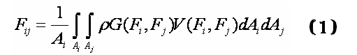
The algorithm for computing the form-factors between faces in the scene is derived from the definition of the rendering equation. The rendering equation itself is the matematical representation of the total light reflected from a given face integrated over the amount of incoming light from each other face in the scene, and is shown below as equation (1).
Analysis of the rendering equation shows that the amount of light reflected from the face Fi is not only dependent on its color and the amount of light incoming from the entire scene, but also depends on its size. This can easily be seen to be an issue if this equation is used to represent the amount of light being emitted from a point light source, because such a point light source lacks any area at all. It is for this reason that a new equation must be derived in order to properly factor the light emitted from point light sources into the total lighting for the scene.
Since the simulated environment we are working with does not exist in a completely mathematical construct, it is necessary to discretize the rendering equation in order to derive a useable algorithm. This process also allows us to find the source of the discrepancies which are conflicting with the point light sources in the scene. The most relevant assumption about the environment to the discretization of the rendering equation is that rather than integrating over infinitesimally small areas dAi and dAj, the scene is already subdivided into the smaller faces which we will use to represent these 'small' parts of the larger plane. Adapting the rendering equation to reflect this assumption, the equation becomes:
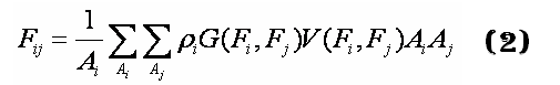
Now, it is easy to see that since we are trying to calculate the light emitted from the given face Fi i is fixed, and the summation over Ai only has one term. Additionally, since the Ai term is common to every element over the summation of each Fj (every other face in the scene), this term can be factored out and, lo and behold, it cancels out the inverse Ai term in front, and the equation takes the form:
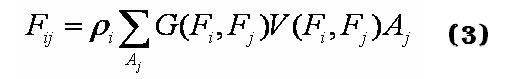
This form indicates that the amount of light leaving the point light source and entering the scene is dependent on the color of the light as well as the geometry between the face and the light (G(Fi,Fj)) and whether or not the face lies within the range over which the light source distributes its light (this includes whether or not the path from the light source to the face is blocked by another object. The amount of light also depends on the size of each other face in question. Thinking logically about what these terms in the equation mean to our environment, we can make a few assumptions about the geometry of the light.
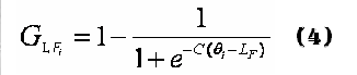
For the purposes of this project, the implementation of the point light sources as spotlights satisfies the needs of the scene, since a non-spotlight point light source can be generalized as a spotlight which does not focus its beam. As with any light source, it is necessary to specify the light's position (LP) and orientation (LD) within the scene, as well as the amount of light (and color) being emitted (LC). These are the basic requirements for any light within the scene, and are usually specified by the particular face's position and orientation in the case of a patch light source. Unique to spotlights is the angle over which the light is distributed, measured from the spotlight's direction (FD) - I will refer to this angle as the 'focus' (or focusing) of the light (LF). Using these variables to describe the light source, it is possible to describe the amount of light incident on any face within the scene using a function for which the light drops off as the angle to the face (with respect to FD) surpasses the focus of the light. In order to provide an animation to the light, it also stores a rotational velocity around each of the three primary axes. A geometry function chosen in such a way also incorporates detection as to whether or not the face lies within the beam. For my implementation, this funtion was chosen to be:
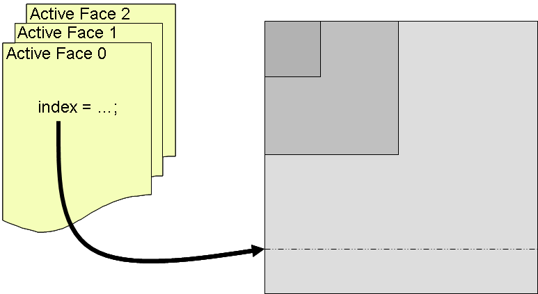
The implementation of spotlights alone is not enough to guarantee that they will be sufficiently rendered within the scene. Due to the resolution of the mesh used to represent the scene, it is entirely possible that the spotlights will not be rendered as the ellipsoid which they should appear as. As a solution to this problem, a quad-tree mesh allows for faces which are partially within the beam of light from a spotlight to be subdivided such that the amount of space missing (or extra space added) to the spotlight's image on a face is reduced. A quad-tree data structure allows the mesh to be initialized and subdivided to the maximum subdivision level, then it is possible to render the scene from a higher level representation so that the number of form-factor calculations can be kept to a minimum while maximizing the detail in those areas that need it the most. The image below shows how a large mesh can be refined to preserve small details in the most relevant areas.
The implementation of a quad-tree isn't too complex by nature. There is a highest level layer of faces which serves as the base implementation for the mesh. Further levels of resolution can be added to the mesh by subdividing each face into four children, each of which is pointed to by the parent face. The parent face must also contain some method with which to indicate whether the face has been subdivided (or if the child faces are active) - if so, the child faces are used to represent their patch in the mesh; if not, the parent face is used.
Due to the differences between the quad-tree mesh respresentation and the standard representation, it is not possible to simply store a matrix of the form factors that can be used for the computation of the radiance values. Since the mesh now contains not only those faces active in the current rendering of the scene, but also the faces which are currently disabled (either because their children are enabled, or because one of their parents are), a solution must be implemented that allows the form-factors to be accessed from the table of form-factors which holds the information for the entire mesh. A simple solution to this problem is for each face to keep track of its index, unique to all faces in the mesh. This then allows for the form-factors for this face to be read from the master form-factor table.
Since the mesh changes between each frame, it makes sense to maintain a list of the active faces within the mesh so that the information about these faces can easily be retrieved for computing their radiance values and for rendering. Having stored all the active faces within a list, since each face has its index in the master form-factor table stored within, it is trivial to retrieve the form factor between any two faces from the master form-factor table. Thus, by using these master indices to retrieve the form factors between any two faces, a solution for the radiance values of each face can be obtained with minimal modification to the standard Gauss-Seidel algorithm. Also, since all active faces are now conveniently stored within a list, it is a simple task to iterate through the list and render each face.
Computation of the form-factors is the most time intensive portion of the simulation, since it requires computing multiple aspects relating to the orientation of each two faces in the scene. The most important computation in determining the form-factor between any two particular faces is determining whether the faces are obstructed by another face in the mesh. The computation time for this value is essentially fixed for the mesh, since it requires iterating through every face in the mesh to determine if that particular face obstructs the path between the original two faces. However, by implementing a partitioning tree in order to better organize the faces within the mesh, it would be possible to reduce the number of faces which must be iterated through in order to determine whether the two faces are occluded by another face in the mesh. The next most significant computations relating to determining the form-factors between the faces are are the distance between the faces and their orientation with respect to each other. This computation cannot be easily eliminated from the algorithm, but it can be seen that this computation requires knowledge of the vertices of the face, which is used to then compute the centroid (position) and the normal of the face. By only computing these values the first time iterating through the faces in the mesh, storing the resulting positions and normals of each face eliminates the need to recompute them every time a form-factor is computed to any particular face. The reduction in computation time resulting from this modification to the algorithm is minimal, but it can be seen that this is still a useful optimization.
The most significant optimization that was applied to the form-factor computation was the reduction of the number of form factors that must be calculated by half. This was made possible by a symmetry inherent in the form-factor computation itself. It can be seen from the simplified form of the rendering equation (Eq 3), that the amount of light reflected from a given face (due to the light emitted from the other faces in the scene) is due to the geometry between the two faces, the area of every other face in the scene, and the color of the face itself. Since the face's color is unique to the face itself, this value can be incorporated only when necessary (during the radiance solving portion of the simulation). The geometry between the two faces is a symmetric value (meaning that the geometry between face i and face j is the same as the geometry between face j and face i. This can be seen the breakdown of the geometry equation, shown below.

Using this symmetry to our advantage, the geometry must only be computed for half the number of form factors (since the geometry between Fi and Fj is the same as the geometry between Fj and Fi, and doesn not have to be computed a second time). It can also be logically deduced quite easily that if it is not possible to see Fi from F j, then it is not possible to see Fj from Fi. Thus, the only differentiating factor between FFij and FFji are the areas of Aj and Ai, respectively. This makes it possible to simply iterate through increasingly less combinations of faces as the computation progresses, ultimately resulting in half the number of form-factors which must be computed.
The table below outlines the differences in runtimes after each of the aforementioned modifications to the form-factor computation algorithm. Due to the extremely fast computation time when the number of faces within the mesh is small, the computation times when the number of faces is 6 do not accurately reflect the resulting decrease in computation time. It can be seen from this test data that the effect of saving the information about each face is roughly a 3-4% decrease in computation time, whereas the half-triangle implementation resulted in about a 47-50% decrease. It seems logical that the reduction due to half-triangulation of the form-factor computation may result in more than a 50% decrease due to overhead which is incurred by performing more computations.
| Version No. | ||||
| 6 faces | 24 faces | 96 faces | 384 faces | |
| v0.0 Basic Implementation | 0.00276 | 0.05700 | 3.72020 | 240.49940 |
| v0.1 Information Storage | 0.00333 | 0.05600 | 3.61210 | 229.10837 |
| v0.2 Half-Triangulation | 0.00143 | 0.02820 | 1.69725 | 111.25110 |
Due to the fact that the spotlights stored within the mesh have zero-area, it makes sense that they would not be stored as faces. This poses the question of how to distribute their light if they are not involved in the form factor computations. By implementing a solution similar to that described in Keller's "Instant Radiosity" paper, the radiance values for the faces that lie within the spotlight are set prior to the radiance computation. This effectively treats those faces as emitters whose emittance is equal to the amount of light reflected from the face solely due to the incoming light from the spotlights. The results of the radiance computation accurately reflect the light due to the spotlights as a result of this solution.
After implemeting adaptive mesh subdivision, the form factors for all the active faces are no longer stored within a single table. This requires that a new method be used for normalizing the form-factors before they are used for anything. In order to normalize the form-factors, each form-factor is divided by the sum of the form-factors for a given face. This procedure ensures that the amount of light being distributed throughout the scene from a particular face is truly the amount of light being reflected from the face. After reconstituting the list of active faces for the given frame, the form factors between each active face are computed, taking advantage of the fact that the form-factors are already in memory at this point, it is simple to add the newly computed (or read from the master form-factor table) form-factor's value to a stored value for the sum of both face i and face j (the two faces involved in the computation of the form-factor in question). Once all form-factors have been computed, these sums can then be used to normalize the form-factor as it is used in following computations.
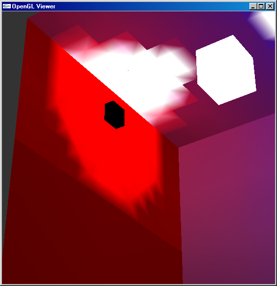
Another problem which arose from the implementation of the adaptive mesh subdivision scheme was the failure of the previous interpolation method to accurately interpolate values between adjacent faces of different levels in the mesh. Due to the difference in resolution, it is not possible for the lower resolution face to accurately render detail comparable to the higher resolution face adjacent to it. This results in blocky interpolated values which are easily noticable in the following image. By forcing the rendering of the highest resolution cells, with radiance values derived from the parent faces, the effects of this issue could be reduced, but due to time constraints, I am unable to submit the findings of this solution.
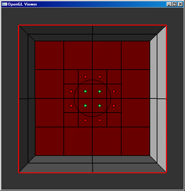
Additional blocky artifacts are caused within the scene by the manner in which the faces of the mesh are subdivided around the spotlights. If any vertex of a face lies within the spotlight and at least one lies outside the spotlight, the face is subdivided to provide a better resolution for the rendering of the image of the spotlight. However, if the resolution provided for spotlight subdivisions is not great enough, it is quite possible that none of the faces which were subdivided will be lit by the spotlight in the final rendering. This is mainly due to the implementation of the spotlight. When the radiance values are initialized from the spotlight (before the radiance computation is performed), the contribution to a particular face is determined using the centroid of that face. Since it is possible that the face is partially within the spotlight, but that the centroid may not be within the spotlight, unneccesary subdivision of certain faces is possible, and the mesh may not only appear blockier than it should, but more form-factors than are necessary will be computed, thus slowing down the simulation. By weighting the initial radiance within a face by the number of vertices within the spotlight, the final solution would more accurately reflect the subdivided mesh in the vicinity of the spotlight.
After implementing these many techniques to not only incorporate dynamic point lighting within the scene, but also speed up the form-factor computations as well as minimize the amount of form-factors which must be calculated, the environment is rendered much more efficiently than at the onset of the project. The number of form factors which must be calculated is still highly dependent on the level of subdivision of the mesh, but by incorporating two different levels of subdivision that can be specified by the user, the amount of detail preserved in the areas of the spotlights can be increased without a global increase in the number of form-factors which must be computed. Prior to the animation of the scene, the form-factors for every initial active face must be computed - this delays the rendering of the environment until these computations have completed, but is a necessary overhead which cannot be avoided. Once the animation has begun and the spotlights begin to move throughout the scene, additional form factors must be computed between the faces which are becoming active due to local mesh subdivision in the vicinity of each spotlight. This results in an initial runthrough of the simulation that takes longer than normal due to the computation of these form-factors. However, assuming the spotlights make it back to their original position, the form-factors computed during the initial computation run do not have to be recomputed, as it is possible to simply read them from the form-factor table. Also, in order to avoid redundant time intensive computations being run every time a particular simulation if animated, the form factor table is saved to disk (assuming the application terminates normally).