Secondary Storage and Indexing
Overview
- Databases are (mainly) optimized for data that is too large to fit in memory.
- How data is stored on secondary storage is crucial for understanding:
- how data is accessed to respond to queries and modify data
- how indices can help speed up queries and the various performance trade-offs in using indices in mixed workflows.
- We will talk briefly about disk technology, storage of data on disk and then discuss various index structures.
Secondary Storage
Data is often stored in hard disks, often there is a trade off:
Magnetic disks are cheap and fast for certain type of access and slow for others
They are not becoming much faster over time, but denser with lots of capacity
Solid state drives (SSD) are fast for most access types but much more expensive (though catching up), has less power draw
Price difference is changing (about twice as expensive per TB), however most SSD drives tend to be smaller in max capacity
SSD is not likely to replace magnetic disks anytime soon, but hybrid solutions will exist.
From now on, we will use the term disk to refer to magnetic disks but discuss differences when we can.
Disk Access
Databases are generally large data stores, much larger than available memory.
Data is stored on disk, brought to memory on demand for operations.
All operations are performed in memory.
If necessary, after an update operation, modified pages are written back to disk to make changes permanent.
A disk page or disk block is the smallest unit of access, to read and write.
A disk page typically is 1K - 8K.
Data Organization
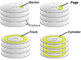
A disk contains multiple platters (usually 2 surfaces per platter)
Usually, the disk contains read/write heads that allow is to read/write from all surfaces simultaneously
A disk surface contains multiple concentric tracks
The same track on different surfaces can be read by different heads at the same time, this unit is called a cylinder
A track is broken down to sectors, sectors are separated from each other by blank spaces
A sector is the smallest unit of operation (read/write) possible on a disk
A disk block is usually composed of a number of consecutive sectors (determined by the operating system)
- Data are read/written in units of a disk block (or disk page)
- A disk block is the same size as a memory block or page.
Reading a disk page
Reading a page from disk requires the disk to start spinning
Disk arm has to be moved to the correct track of the disk: seek operation
The disk head must wait until the right location on the track is found: rotational latency
Then, the disk page can be read from disk and copied to memory: transfer time
The cost of reading a disk page:
cost = seek time + rotational latency time + transfer time
Multiple pages on the same track/cylinder can be read with a single seek/latency.
Reading M pages on the same track/cylinder:
cost = seek time + rotational latency time
       + transfer time * (percentage of disk circumference to be scanned)
A high end disk example
Consider a disk with:
16 surfaces
2^16 tracks per surface (approx. 65K)
2^8=256 sectors per track
2^12 bytes per sector
- Each track has = 2^12 * 2^8 =2^20 bytes (1MB)
- Each surface has = 2^20 * 2^16 = 2^36 bytes
- The disk has = 2^4 * 2^36 = 2^40 byte = 1 TB
Reading a page
- Typical times:
- 7200 rpm means one rotation takes 8.33 ms (in the average, 1/2 of the disk needs to be rotated before the correct location is found, 4.17ms)
- seek time between 0 - 17.38 ms (in the average, 1/3 of the disk surface is scanned = 6.46 ms)
- transfer time for one sector : 8.33/256 = 0.03 ms
Reading a page
Reading a page of 8K (2 sectors):
Sequential scan: 1 seek + 1 rotational latency + 2 sector transfer time
6.46 + 4.17 + 0.03 * 2 = 10.69 ms
Random access: Reading 100 consecutive pages on the same track:
6.46 + 4.17 + 0.03 * 10 = 13.63 ms
The lesson: Put blocks that are accessed together on the same track/cylinder as much as possible
Sequential scan: access of pages on the same track (or same cylinder requiring a single seek) consecutively: single seek and rotational latency, then transfer data, very fast.
Random access: In the worst case, as many seeks as the number of pages, very costly.
Important messages: Depending on how data is stored, disk access times can vary greatly!
Disk scheduling
- The disk controller can order the requests to minimize seeks
- When the controller is moving from low tracks to high tracks, serve the next track request in the direction of the movement, queue the rest
- The method is called the elevator algorithm
Solid State Drives
Magnetic disks can have significant different read times depending on how different data blocks are stored.
On high update systems, it might be hard to store information in consecutive pages or same cylinder (fragmentation).
Solid state drives do not have this type of extremely different access times. No moving parts, less power usage and no seek penalty.
However, still significantly slower than memory access.
Reliability of both is similar, though SSD’s are slightly worse at the moment.
Reliability - RAID
- Speed of access and reliability of disks can be increased by simply using multiple disks.
- RAID: Redundant arrays of inexpensive disks is a simple theory of using multiple disks to increase both speed of access and reliability of disks.
- RAID can be implemented using a hardware controller or a software controller.
- Different levels provide different solutions at different price points. We will see only some examples.
RAID-0
Striping of data to distribute it to multiple disks.
Example with 4 disks:
Disk 1 has pages 1,5,9
Disk 2 has pages 2,6,10
Disk 3 has pages 3,7,11
Disk 4 has pages 4,8,12
Reads are faster as now multiple page reads can be from multiple disks in parallel.
Writes are faster for the same reason.
No redundancy. If one of the disks fail, the data stored in the whole array is unrecoverable.
RAID-1
- Mirror data to two disks
- Reads are twice as fast as we can read from any disk.
- Writes are slowers because data must be written to both disks and the write is not complete until both writes are complete (cost of synchronization).
- Failure of one drive leads to no data loss because the second drive has the complete copy of data.
RAID-4
Calculate a parity of N disk blocks as a new block of data. The simplest parity is a checksum:
The checksum is 1 if the number of 1’s in the given sector is odd, and 0 if the number of 1’s is even.
Page 1 Disk 1:  10101011
Page 2 Disk 2:  01000101
Page 3 Disk 3:  10010110
Page 4 Disk 4:  10011000
Page   Parity:  11100000
Store each page and parity on a separate disk. The above solution requires 5 disks.
Reads are faster due to potential parallel reads (same as RAID-0).
Writes are slower because of the need to update the parity as well as the data disk.
Note: You do not need to read all data pages at the same location, just the new data disk and parity, and update parity.
Page X Disk Y old value:      10011000
Page X Disk Y new value:      00010010

Old parity for page X:        11100000
Changes for parity:           01101010
Keeping all other data pages the same, we only need to flip the parity in bit locations page X has changed.
Redundancy: If there is a 1-disk failure, we can still recover the lost data by reading all the remaining data including the parity.
Page 1 Disk 1:  10101011
Page 2 Disk 2:  01000101
Page 3 Disk 3:  ------------- CRASHED
Page 4 Disk 4:  10011000
Page   Parity:  11100000
Page X of Disk 3 can be reconstructed by computing the parity of all the readable data.
Reads are slower when operating with a missing disk. All data is lost in case of a second disk failure.
RAID-5
Same as RAID-4, for each page compute a parity page, but change how parity is stored.
Disk 1       Disk 2       Disk 3        Disk 4       Disk 5
-----------  -----------  ------------  -----------  ------------
Page 1       Page 2       Page 3        Page 4       Parity 1-4
Parity 5-8   Page 5       Page 6        Page 7       Page 8
Page 9       Parity 9-12  Page 10       Page 11      Page 12
Page 13      Page 14      Parity 13-16  Page 15      Page 16
Reads are the same as RAID-4. Redundancy is the same as RAID-4.
Writes are faster because the parity disk changes depending on the page being written. The parity disk does not become a bottleneck as in RAID-4.
RAID-6+
Higher levels of RAID use other parity methods, such as a 2-bit Hamming-code parity stored in 2 redundant disks.
Such methods can handle up to two disk failures without loosing data with increased read performance similar to lower levels of RAID.
Tuple storage on disk
A disk page typically stores multiple tuples.
Large tuples may span multiple disk pages.
Many different organizations exist.
The number of tuples that can fit in a page is determined by the number of attributes and the types of attributes the relation has.

- Header information contains LOG data: when the data on that page was updated (as well as other control information).
- The offset information can tell where each field in the tuple start for variable length attributes.
Tuple Addresses
A disk page typically stores one or more tuples.
Tuples have a physical address which contains the relevant subset of:
Host name/Disk number/Surface No/ Track No/Sector No
- Physical address tends to be long
- Tuples are also given a logical address in the relation,
- A map table stored on disk contains the mapping from the logical address to physical address
When tuples are brought from disk to memory, its current address becomes a memory address
Pointer swizzling is the act of changing physical address to the memory address in the map table for pages in memory
Indices as Secondary Access Methods
A table is a primary access method. To find a tuple in the table, we need to search the whole table.
An index is a secondary access method, allowing us to search the table for a search key.
The search key can consist of multiple attribute
The index contains pointers to tuples (logical address)
The index itself is also packed into pages and stored on disk.
Notice the big difference between a data structure you may have seen in other classes:
- Indices allow a new access method to the same data
- Indices are stored on disk, not memory.
- Indices need to be brought to memory to be used as well.
Dense vs. Sparse Indices
- The index is called dense if it contains an entry for each tuple in the relation.
- An index is called sparse if it does not contain an entry for each tuple.
- A sparse index is possible if the addressed relation is sorted with respect to the index key.
Dense Index Example
Suppose table T(A,B) is stored in two pages:
Table T P1:  (t1:[21,a], t2:[12,b], t3:[8,c], t4:[4,d])
Table T P2:  (t5:[31,e], t6:[35,f], t7:[10,g], t8:[1,h])
Suppose we create an index I1 on T(A) which is also stored in two pages:
Index I1 PX:  (1,t8/P2), (4,t4/P1), (8,t3/P1), (10,t7/P2), (12,t2/P1)
Index I1 PY:  (21,t1/P1), (31,t5/P2), (35,t6/P2)
Note the following:
The index may be able to store more information in each page because it only stores the search key and the pointer to tuple.
If we were to search for a B value, the index is not useful.
If we search for an A value but return B, then the index is partially useful:
SELECT B FROM T WHERE A=4;
To answer this query, we can search the index to find that this value is stored in tuple t4. Then, we need to read t4 to read and return the B value.
Cost involves the cost of scanning the index and then reading the relevant data pages from the relation.
Sparse Index Example
Suppose the above table T is stored in sorted order of B explicitly.
Table T P1:  (t1:[21,a], t2:[12,b], t3:[8,c], t4:[4,d])
Table T P2:  (t5:[31,e], t6:[35,f], t7:[10,g], t8:[1,h])
We can create a different type index I2 on T(B):
Index I2 Page P5: (_,P1), (e,P2)
This index says that to find values less than e for B, go to page P1. Otherwise go to P2.
We will not necessarily know if a B value is stored by simply looking at the index.
However, the index is much smaller, making it less costly to search.
Multi-level Indices
You can build multi-level indices:
- Lowest level is the index pages pointing to tuples (dense or sparse)
- Upper levels point to the lower level index pages (often sparse given the index is sorted by the search key)
We will convert the above index I1 to a multi-level index.
Index I1 PX:  (1,t8/P2), (4,t4/P1), (8,t3/P1), (10,t7/P2), (12,t2/P1)
Index I1 PY:  (21,t1/P1), (31,t5/P2), (35,t6/P2)

Index I1 PZ:  (_,PX), (21,PY)
To search this index, we start at the top level of the index (page PZ), which tells us which index page at the lower level to go to. Then, we find the necessary tuple and read the tuple from disk if necessary.
SELECT B FROM R WHERE A=31

Read index page PZ: Decide we must read index page PY
Read index page PY: Decide we must data page P2
Read data page P2: Find tuple t5, return the B value: f.
Other types of indices
- An index organized table is an index that also stores the data.
- Index organized tables in Oracle and clusters in Postgresql.
- This type of index is often sparse. It can be multi-level depending on the type of index.
B-tress
- Note while we are going to use the term B-trees, the type of B-trees we will use are often referred to as B+-trees in other places.
- B-trees are like binary search trees, except instead of 2 (binary), they have often between n/2 to n entries.
Basic properties of B-trees
- Each node on a B-tree is mapped to a disk page
- A B-tree is of order n (but n may change depending on different properties)
- Leaf nodes:
- Leaf nodes point to the next node in the leaf, called a sibling node.
- A leaf node can contain at most n tuples (key values and pointers) and 1 additional pointer to the sibling node.
- A leaf node must contain at least floor((n+1)/2) tuples (plus one additional pointer to the next sibling node.
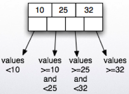
- Internal nodes:
- An internal node can contain at most n+1 pointers and n key values.
- An internal node must contain at least floor((n+1)/2) pointers (and one less key value), except the root which can contain a single key value and 2 pointers.
- A B-tree created on a search key A will have (dense) leaf nodes
sorted by A. The internal nodes will be sparse indices to the lower
levels.
- Often B-trees are secondary structures, so we will assume so. It is possible that they are used as part of an index organized table, but we will not go into details in the discussion below.
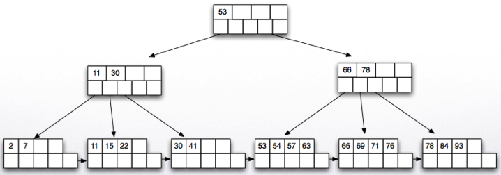
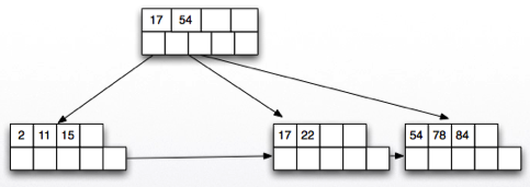
- Example B-tree:
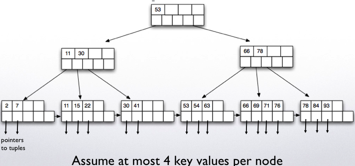
B-tree example
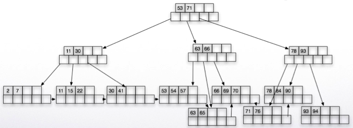
- Suppose n = 3
- Each leaf node will have at least 2 and at most 3 tuples.
- Each internal node will point to at least 2 and at most 4 nodes below (and hence will have between 1 and 2 key values).
- Suppose n = 99
- Each leaf node will have at least 50 and at most 99 tuples.
- Each internal node will point to at least 50 and at most 100 nodes below (and hence will have between 49 and 99 key values).
- The root can have 2 pointers and 1 key value in the least.
Searching in B-trees
Index on a single attribute A
Search for equality (A=x)
Given an index on attribute A find all tuples with A = x

Start at root

Repeat until leaf node is reached:
  Find the first key value that is greater than x
  Follow the pointer just before this key value

Find if leaf node contains the key value x (if not, return empty)

Find and return the tuple id
Search for range:
Given an index on attribute A find all tuples in the range x1 <= A <= x2:

Start at root

Repeat until leaf node is reached:
   Find the first key value that is greater than x1 and less than x
   Follow the pointer just before this key value

Repeat until leaf node contain values greater than x2:
   Find all entries in leaf node in the given range
   Retrieve the next leaf node (sibling pointer) and continue

Return all found tuple ids
Index on multiple attributes A,B
An index on multiple attributes like A,B will sort tuples first by A and then by B
Queries:
A = x AND B = y: same as searching A=x for index on A
A = x AND y1 <= B <= y2:
search for first value with A=x and y1 <= B <= y2:
scan leaf nodes to the right following sibling nodes
A = x
search for first value with A=x (regardless of B)
scan leaf nodes to the right following sibling nodes
x1 <= A <= x2 AND B = y
search only for x1 <= A
scan leaf nodes for x1 <= A <= x2 following sibling nodes
for the nodes that I find, check if B=y, and if so,
put in the output
B = y
find the first leaf node, scan all leaf nodes following
sibling nodes, for each tuple, if B=y, add to the output
[index only scan]
Notice that B-trees allow many different types of search on equality and range. However, ranges in the second attribute are not useful unless an equality in the first attribute is given.
Index only search
Given
select A from R where A < 120 and A > 10
and an index on R.A:
Scan the index for matching tuples as before and return the found A values (no need to read the tuples from disk)
Index partial match
Given an index on R(A,B) (index is sorted on A first and then on B)
select C,D from R where A > 10 and A < 100 and B=2
Scan index for the range A > 10 and A < 100, and for each matching tuple check the B value, read matched tuples from disk for C,D attributes
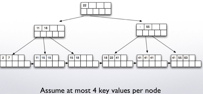
B-trees with duplicate values
- If the B-tree is built on a key value that may contain duplicates,
build the index in an identical way, except:
- The non-leaf node pointing to leaf node contains the key value of the first node that is not repeating from the previous sibling
- If there is no such key, then a null value is stored at this location.
Insertion
Insertion involves two steps:
- Insert starting from the root
- Then check if the insertion resulted in the root being split
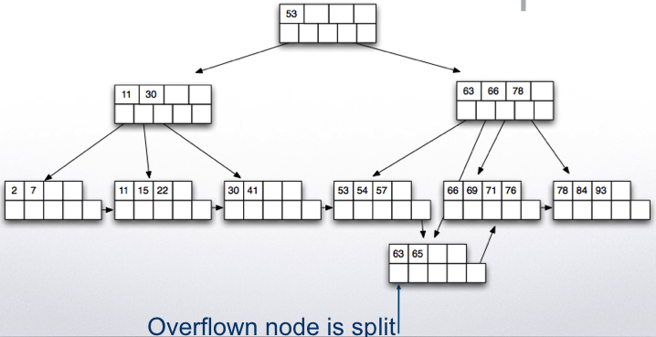
If insertion of a node that causes the node to be over full (with more than n key values for leaf or n+1 pointers for internal nodes), then split the node.
Insertion(root, newval)

   node = leaf node to insert the newval starting with root
   result = insertion_helper(node, newval)
   if result != null : ##the root was split
      newroot = new_node
      point from newroot to root
      point from newroot to result
      root = newroot
   return root

Insertion_helper(node, newval)

   If there is space in the node
      Insert and return null
   Else
      Create a new node (a new disk page)
      Distribute entries for the current node to the two nodes evenly

      recursively insert a pointer to the new node in the
      parent node

      if the parent is full, then split the parent (distribute
      pointers and key value evenly) and recursively insert to
      parent

      if root has split, return the new node created
Insertion example:
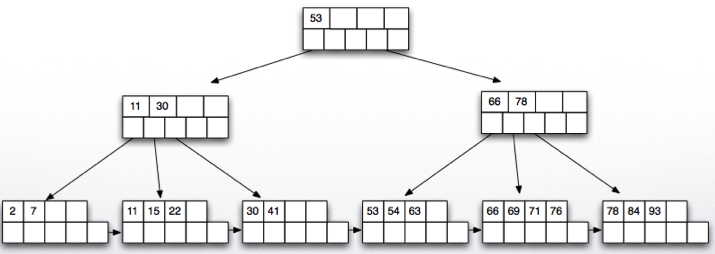
- Insert 57:
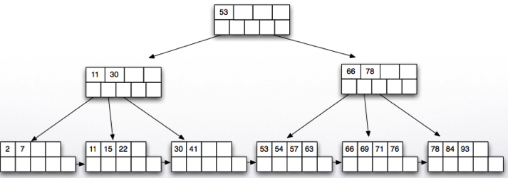
- There is space in the node, we are done!
- Insert 65:
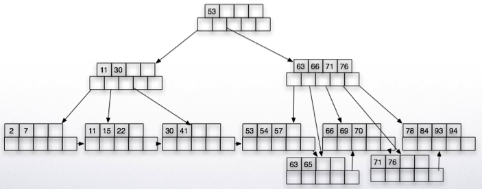
- Insert 70 and 94, one more node split:
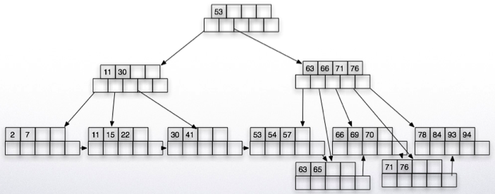
- Finally, insert 90 which will cause the parent to split.
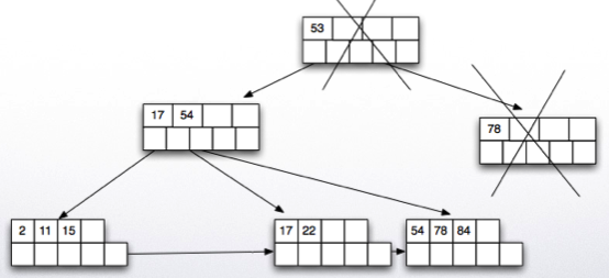
Deletion
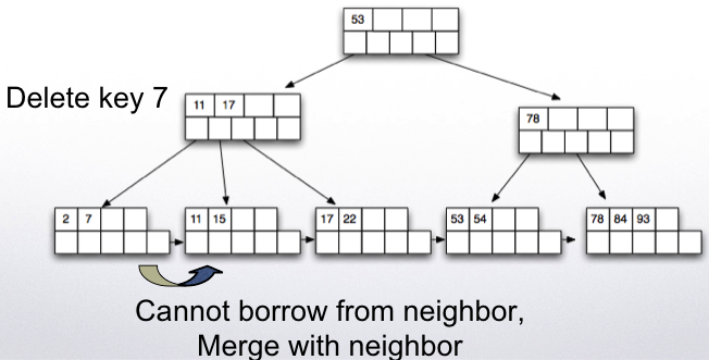
Deletion works in reverse. If after removing a key value/pointer, the node is less than half full, then we try to borrow from a sibling.
If this is not possible, then we merge with a sibling node.
Call deletion helper from root
If root now points to a single node in the next level,
delete root and make the next node the new root

Deletion helper:

   Find the key value to be deleted and if it exists delete it
   and update the parent node key value if necessary.

   If node is less than half full
      if it is possible to borrow a key value (leaf
      nodes ) or a pointer (for internal nodes) from a sibling:
         Borrow and adjust key values and done.
   Else:
      merge with one of the siblings and
      delete a pointer from the parent recursively
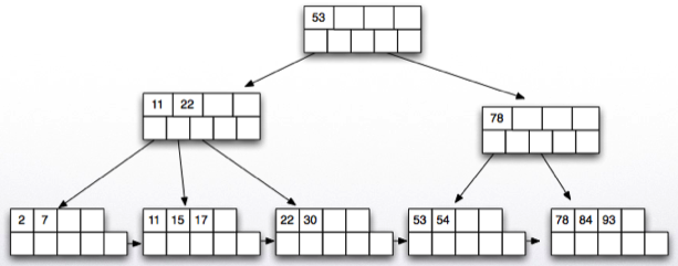
- Delete key 30.
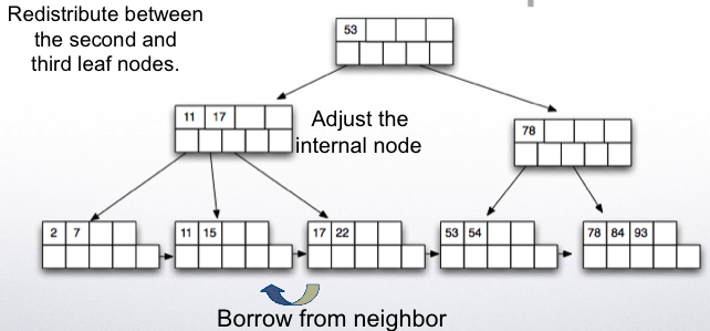
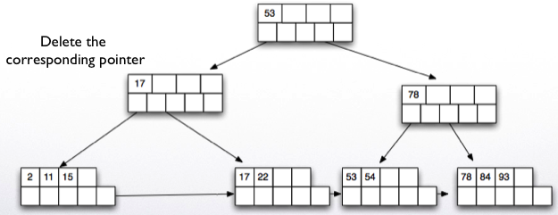
- Delete key 93.
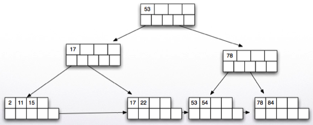
- Delete key 53.
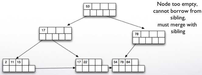
- Results in deletion of the root node.
B-tree example
Given: - disk page has capacity of 4K bytes - each tuple address takes 6 bytes and each key value takes 2 bytes - each node is 70% full - need to store 1 million tuples
Leaf node capacity - each (key value, tuple address) pair takes 8 bytes - disk page capacity is 4K, so (4*1024)/8 = 512 (key value, rowid)
pairs per leaf page
in reality there are extra headers and pointers that we will ignore
Hence, the maximum number of points for the tree is about 256 (and 255 key values)
If all pages are 70% full, each page has about 512*0.7 = 359 pointers
To store 1 million tuples, requires
1,000,000 / 359 = 2786 pages at the leaf level
2789 / 359 = 8 pages at next level up
1 root page pointing to those 8 pages
Hence, we have a B-tree with 3 levels
B-trees vs. R-trees
B-trees are useful for range searches, but not for searches along two axes:
x1 <= A <= x2 and y1 <= B <= y2
In this case, the second range is not useful in limiting the number of nodes searched.
When searching for spatial data, a common query is finding all points (x,y) values in a range as the one above.
To facilitate such searches (as well as other special queries like nearest neighbor searches), R-trees are introduced.
An R-tree is similar to a B-tree except each key value in an internal node is a rectangle and contains a pointer to values and rectangles within that rectangle.
- Postgresql GIST structures allows you to implement R-trees.
Bitmaps and Inverted Indices
When indexing text valued attributes, it is necessary to first preprocess the text fields to find all words within.
Then, a listing file for each word is created:
word-> (tupleid, location within tuple), ...

e.g.

pizza -> t1,2 t1,5 t3,4 t5,12
Then each inverted listing is compressed for storage.
A Boolean keyword query is processed by bitmap operations (bitwise AND, bitwise OR) over these vectors.
- Postgresql GIN structures are used for this purpose and text querying.
- Other open source implementations of inverted files such as Apache Lucene project exist.
- Google main index is a distributed and replicated inverted index over the Web documents.
Primary vs Secondary Indices
As mentioned earlier, an index structure can be secondary:
data pages containing a table

index pages containing pointers to tuples
in these data pages at leaf level
Primary B-tree indices are also possible
internal nodes contain pointers to levels below

leaf level contains data pages for the table
There can only be a single primary index.
- Use clusters in Postgresql to generate primary indices.
Hashing
Hashing is often a primary index method.
Given a hash function h with K values and an attribute A
Allocate a number of disk blocks M to each bucket
For each tuple t, apply the hash function h(t.A)=x.
Store t in the blocks allocated for bucket x.
To search on attribute A (select * from r where r.a=c)
Apply hash function, h(c)=y.
Read the buckets for y to find value c.
Search half the pages for that bucket in the average and all the pages in the worst case (M/2 pages in the average)
Search on another attribute:
- Hash does not help, search all the disk pages
Insertion cost: 1 read and 1 write (find the last page in the appropriate bucket and store)
Deletion/Update cost: M/2 (search cost) + 1 to update
If a bucket has too many tuples, than the allocated M pages may not be sufficient
- Allocate additional overflow area
- If the overflow area is large, the benefit of the hash is lost
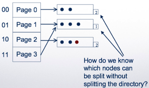
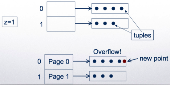
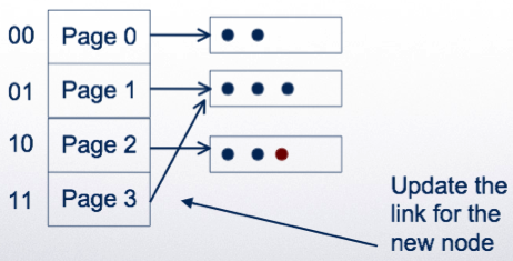
Extensible hashing
- The address space of the hash (K) can be adjusted to the number of tuples in the relation
- Use a hash function h
- But, use only first z bits of the hashed value to address the tuples
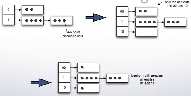
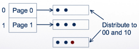
- If a bucket overflows, split the hash directory and use z+1 bits to address
- Example: using a single bit to address:
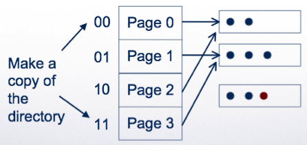
- Double the directory
Linear hashing
The addressing is the same, but we allow overflows
We decide to split based on a global rule
- Example: if number of pages/number of tuples > k %
Split one bucket at a time
The bucket split is the next one in sequence it may not be the one that has overflow pages eventually all buckets will be split