Query Processing#

Overview#

Databases implement relational algebra operators as the basic units of operation. The implemented operators are bag versions of the relational algebra, to be in sync with SQL (plus include a group by operation).
A logical query plan is represented as a query tree where the relations are leaves of the tree and the algebra operators are intermediate nodes.
A single algebra operation can have many different implementations. For example, joins can be implemented using sort-merge-join, hash-based-join, block-nested-join, etc.
The physical implementation plan of a query is a query tree with additional information, the amount of memory reserved for each node and the specific implementation of the given operation.

We will use M to denote the number of blocks available to a query or operation.
Given a query, there may be many potential query trees. Each has an associated cost that can be estimated before the query is executed.

The dominant cost is always the total number of disk pages read and written to execute the query.
Note that CPU complexity of a query is going to be disregarded (i.e. the complexity of the algorithm once the data is in memory) due to the following reasons:
- The cost of reading/writing data is much higher than any operation in memory. So, the donimating cost is disk access.
- We assume each algorithm is implemented as efficiently as possible.
- It may not even be possible to bring all the data for a query in memory at once, which may result in the data being read multiple times.

Disk Access Process (Overly Simplifed)#

Remember that to process any data, it must be first brought to memory.
Some DBMS component indicates it wants to read record R
- File Manager:
  
  Does security check
  
  Uses access structures to determine the page it is on
  
  Asks the buffer manager to find that page
- Buffer Manager
  
  Checks to see if the page is already in the buffer
  
  If so, gives the buffer address to the requestor
  
  If not, allocates a buffer frame
  
  Asks the Disk Manager to get the page
- Disk Manager
  
  Determines the physical address(es) of the page
  
  Asks the disk controller to get the appropriate block of data from the physical address
  
  Disk controller instructs disk driver to do the dirty job

Example query plans#

Let’s us look at a simple query:
```
SELECT R.C,S.E
FROM R,S
WHERE R.B=S.D and R.A=10 ;
```
and two potential logical query trees:

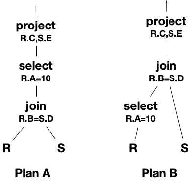
In plan A, we compute the join of R and S first. Then, the selection and projection can be computed over the results of the join.
In plan B, we first select tuples that satisfy the condition R.A. The resulting tuples are then joined with all the tuples in S and then we apply the projection to the resulting tuples.

Iterator Interface#

Each operator in the database is implemented using three main functions:
- open() initializes the necessary memory structures (i.e. M buffers) and/or streams
- getNext() reads data input streams and processes the data until a block full of output is produced or the input is completely processed, puts the output to the output buffer
- close() frees all the structures used by the operator
Since each operator works the same way, we can chain up the operators by using the input buffer for an operation as the output buffer for the operation below.
- If this is the last operation in the query tree, then the output buffer is simply the standard output to the user executing the query.
Certain operations are easy to combine with the previous operation without any additional cost. These are identified as “on-the-fly”. For example, if the tuples are already in memory, any selection and projection operation can be performed in memory.
Certain operations are blocking, i.e. these operations have to be completed before any tuples can be processed by the operations above. For example, sorting and group by are blocking operations unless the relation is already sorted by the relevant attributes.
If the operations are not blocking, then the output of one operation is pipelined into the input of the next operator immediately, producing some output tuples without the query is completed.

Example Execution#

Suppose we are processing the above query
```
SELECT R.C,S.E
FROM R,S
WHERE R.B=S.D and R.A=10 ;
```
by mapping the logical query trees above to more explicit physical implementations:

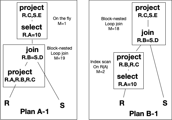
In Plan A 1: To prepare the join operation, we ready R for a scan to fill the memory blocks for the block-nested-loop-join. Once the sufficient blocks are filled, we will start scanning S to compute the join.
- We add a projection to sequential scan of R to keep the attributes needed by the query, which will reduce the size of the relation in memory, which may reduce the cost of the join (if we end up reading S fewer times). This projection is completed in memory as tuples are read and has no additional cost.
- The next() operation for the join will output tuples to the selection operation as soon as joining tuples are found. Hence the join and selection are pipelined, they are not blocking.
- The selection operation reads the tuples output by the join, removes tuples that do not match the join condition and projects the requested attributes. These operations are performed completely in memory and have no additional disk I/O cost.
In Plan B 1: Since we decided to do the selection first, we can use an index for the selection.
- As tuples matching the index search condition are found and read from the disk, we can project the necessary attributes and fill the input buffer for the block-nested-loop join as before.
- We have the index search operation being pipelined into the join, which is combined with the last projection operation. Because of this, there is no additional cost of reading the relation R in the join. The cost of reading R is included in the index scan.

Query Execution Costs#

Often query costs involve the sum of the cost of each operation. However, the costs may incorporate additional costs if we need to write the results of the relations into memory.

../../_images/query_plans_physical_2.png

Let’s assume the following statistics for these relations.

PAGES(R )=1,000
PAGES(S)=5,000
PAGES( PROJECT_(R.A,R.B,R.C) (R ) = 500 
PAGES( PROJECT_(S.D,S.E) (S) = 800

PAGES( PROJECT_(R.B,R.C) (SELECT_(R.A=10) R) = 15

Index on R(A):  200 left nodes 
Selectivity (R.A=10) = 1/100
TUPLES(R) = 20,000

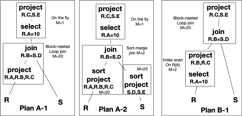
Plan A 1: The main cost is the cost of join because the remaining selection and projection are performed on the fly.
- Block-nested-loop-join: We read R once, 1,000 pages.
- Since we do projection while reading R, we actually need 500 pages space to keep R in memory, which requires us to read S 500/20= 25 times.
- Total cost: 1000 + 25*5000 = 126,000 pages.
Plan A 2: We will sort R and sort S fully , and then compute the join.
- Sort R, read R fully (1,000 pages), project attributes A,B,C and write 500 pages worth of data using M=20 blocks, which is 500/20=25 partially sorted groups. (Cost = 1,500 pages)
- Merge 25 groups into 2 groups using M=20 pages, and 2 groups into 1 group. Read/write 500 pages 2 times. (Cost = 500*4=2,000 pages)
- Sort S: Read S fully (5,000 pages), project attributes D,E and write 800 pages worth of data using M=20 blocks into 800/20=40 partially sorted groups. (Cost = 5,800 pages)
- Merge 40 groups into 2 using M=20 pages and 2 groups into 1 group. Read/write 500 pages 2 times. (Cost = 800*4=3,200 pages)
- Assuming the join is involving unique attributes R.B and S.D, then the sort-merge-join can be done by reading sorted R and S only once, total cost of 500+800 = 1,300 pages.
- Total cost = 1500+2000+5800+3200+1300=13,800.
- Note that the actual cost is likely much lower as the last sort merge steps and the join can be combined, saving 2,600 pages.
Plan B 1: Index scan involves scanning, 200/100= 2 leaf nodes. The scan will find estimated: 20,000/100 = 200 tuples which requires reading 200 pages in the worst case. The cost of index scan is 2+200 pages (plus 1 or 2 for internal nodes that we will disregard).
- Block nested loop does not have any additional cost of reading R since the R tuples are already in memory after the index scan. We simply need to find out how many times S needs to be read for the join.
- Now the resulting 200 tuples from R fit in 15 pages (according to the statistics above), we can complete the join by reading S only once since the join has 20 blocks of memory allocated and all of found tuples of R fits in memory completely. Total additional cost for the join: 5,000 (read S once.)
- Total cost = 202 + 5,000 = 5,002.
In this example, plan B is the clear winner because the selection on R.A is very selective.

Query operators#

In the rest of the course notes, we go over some basic types of operator implementations. Sort and block-nested-loop-join were already covered in the previous section.
Query operators are classified into classes:
- One pass
- Two pass
- Multi-pass
depending on the availability of memory, storage method of the relation (i.e. sortedness for example) and the number of pages it occupies on disk.

One pass algorithms#

The algorithms require one pass over a given relation.
One easy way to think about this is as follows. Suppose we have a unary operation over relation R. If R fits in memory allocated to the query, then we can easily compute the operation in memory. However, many operations do not read all of R to be read into memory either. This is discussed below for each operation.

Duplicate removal#

Given M pages of memory. Let X be 1 page, and Y be M-1 pages in memory.

Read R into X, 1 page at a time.

For each tuple t, check:
   If tuple t is in Y:
      it is already seen, remove t.
   Else
      insert t into Y.

getNext() will read a one block from Y and output. The next time it will be called, we need to process the operation until another block in Y is filled.
This is a one-pass operation only if after duplicate removal, R fits in M-1 blocks.
Not a blocking operation as we can start outputting tuples as long as we can mark them so that we do not return the same tuple more than once.

Group by#

Given M pages of memory. Let X be 1 page, and Y be M-1 pages in memory.

For each group in Y, we are going to keep:
    the grouping attributes
    the aggregate value
       for min, max, count, sum: keep min, max, count,
       sum of the tuples seen so far

       for avg, keep count and sum.


Read R into X, 1 page at a time.
For each tuple t, check:
    If the corresponding group for tuple t is in Y:
         update its aggregates.

    Else
          create a new group for t into Y and initialize its statistics.

This is possible only if all the results fit in Y (M-1) blocks. Blocking operation: we cannot output the tuples until we finish processing all of R.

Set and bag operators#

Bag Union of R and S:

Read R one block at a time and output
Read S one block at a time and output

Set Union of R and S:

Read R and remove duplicates
Read S into the same space and continue to remove duplicates

Set intersection:

Read R, remove duplicates and store into M-1 blocks (section Y).
Read S.
If the tuple is in Y
      output and remove from Y
Else
      discard the tuple

Bag Intersection:

Bag intersection requires that we keep track of how many copies of each tuple there are.

Read R, group by all attributes and add a count for R.
Store into M-1 blocks (Y section).

Read S, for each tuple:
    If is in the Y section
         increment the count for S
    Else
         disregard
Output min of count of R and S.

All set/bag operations are defined similarly. In most cases the algorithm is one pass only if the necessary memory is available.
In general, the cost of one pass the algorithms is PAGES® + PAGES(S) if R and S are being queried, again assuming memory is available.

External Sorting#

A large number of operators can be executed by an intermediate sorting step:
- DISTINCT
- ORDER BY
- GROUP BY
- UNION/INTERSECTION/DIFFERENCE
A limited amount of memory is available to the sort operation

M: the number of memory pages available for the sort operation

PAGES®: total number of disk pages for relation R
If PAGES® <= M, then the relation can be sorted in one pass: read the relation into memory and apply any sorting algorithm. The cost if PAGES® pages.

Sort based duplicate removal#

When a “distinct” projection is needed, we can do the following:

Sort the relation
Read the relation in sorted order
For each tuple:
   If it is already seen
      discard
   Else:
      output

Need to keep in memory the last seen tuple only, so 1 page is sufficient for the operation.

It is possible to combine sort and duplicate removal

Read the relation in groups, remove all unwanted attributes

Sort the tuples in memory, remove duplicates (distinct) and write
the sorted group to disk

Read the sorted group for k-way-merge, during merge remove any
additional duplicates

Sort based projection#

Cost is similar to external sort, but the relation being read in the second stage is reduced in size by removing unnecessary attributes
Tuples are smaller (how many attributes are removed?)
Duplicates are removed (how many duplicates are there?)

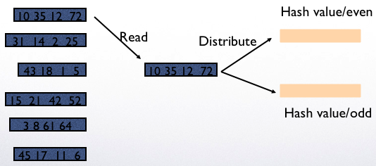
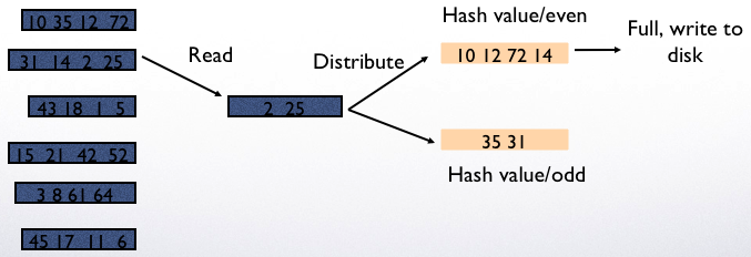
Hash based projection#

To compute “distinct R.A, R.B,…”:

Read all tuples in R and extract the projected attributes

Hash the remaining attributes to buckets 1 … M in memory (and continuously remove duplicates from buckets in memory)

Whenever a bucket in memory is full, write it to disk

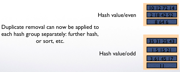
For any bucket that takes up more than one disk page, read it back from disk to memory and remove duplicates within the bucket.
Example: 2 pages for hashing and 1 page for processing

Read and put values into the two buckets

If the bucket needs to be computed before the query executes, it needs to be written to disk.

Once hashing is complete, different operations can be mapped to different buckets and applied independently in each bucket.

Hash based projection#

The cost:

The relation has to be read once for hashing

If all the buckets after reduction are too large fit in a single memory block, then the relation will be written once to disk

If all the disk pages in a single bucket will fit in the M available blocks, then the last step can be performed in one read.

Set operations#

To compute A UNION B (with duplicate removal), we first hash both A and B together and remove duplicates in each bucket separately.
To compute A - B, we hash A and B into the same buckets and then compute A - B to each bucket separately.

Index nested loop join#

Index loop join assumes a look-up of matching tuples for S using an index.

Given R join S on R.A=S.A

Read R one block at a time
   For each tuples r of R
      Use index on S(A) to find all matching tuples
      Read the tuples from disk and join with

If R is not sorted on A, then we might end up reading the same tuples of S many times
- What if A is R’s primary key?
  
  Then, for each A value, we will look up S only once
Cost:
- The outer relation R is read once, PAGES®
- Assume for every tuple r in R, there are about c tuples in S that would join with R (ideal case is c is very small or 0 most of the time)
- Then, for each tuples in R: - We find the matching tuples in S (cost is index look-up, in the
  
  best case one tuple for each level, so h+1 for an index with h levels)
  - Then, if we need attributes that are not in the join, we read c tuples from S (which can be in c pages in the worst case)
  - Total cost is between PAGES® + TUPLES® * (h+1) (if no tuples match or index only scan is fine) and PAGES® + TUPLES® * (h+1+c)

Example:

SELECT S.B FROM R,S WHERE R.A = S.B

Index I1 on S(B) with 2 levels (root, internal, leaf)
PAGES(R)=100, TUPLES(R)= 2000
PAGES(S)=200, TUPLES(S)= 4000

Cost = 100 (for reading R) + 2000*3 (index look up for each tuple of R)

SELECT S.C  FROM R,S WHERE R.A = S.B

Assume statistics are same as above, but we now need to reach
each matching tuple (at most 4000 tuples will match)

Cost = 100+2000*3+4000 (one page read for each matched tuple)

How could this be, there are only 200 pages of S?

Well, if we are not finding all pages that we need to read first and reading each page as we find a match, we may end up reading the pages for S multiple times.

Of course, in reality, you will likely do a lot of reduction of duplicate page requests in memory and improve on this. This is the worst case scenario.

Will we ever do this?

No, we will choose not to use index join for this case, clearly it looks very expensive and we better do some other operation.

Another example:

SELECT S.B FROM R,S WHERE R.A = S.B AND R.B=100

Index I1 on S(B) with 2 levels (root, internal, leaf)
PAGES(R)=100, TUPLES(R)= 2000
PAGES(S)=200, TUPLES(S)= 4000
Suppose only 3 tuples match R.B=100

So, we can:
   Scan all of R to find these 3 tuples (100 pages)
   Read matching tuples from S (3*3)
   Total cost = 109 (using only 2 pages of memory)

   This would cost a lot more in block-nested loop join
   with M=2 (200 pages). So, index join is for cases
   where the outer relation is very small (normally after
   a selection)

Sort-merge join#

Sort both R and S first
Read R and S one block at a time, and join the matching tuples.
Sort merge is similar to Step 2 of the sorting algorithm.
Sort-merge join

Example:

R: [1, 2] [5, 8]    S:[1,5] [6, 7]
Read [1,2] and [1,5] first, join 1.
Read the next block of R, [5,8] [1,5]. Join 5
Read the next block of S, [5,8] [6,7]. No more tuples, done.

If each joining attribute has unique values in R and S, then the join can be performed in a single step without reading each relation once forward, PAGES® + PAGES(S) + the cost of sort
If there are duplicate values, then we must worry about if all the duplicate values from both relations will fit in memory

Example:

R [1,2] [2,2] [2,2] [2,2] [2,2] [2,2] [2,2] [2,2] [2,2][2,3]
S [1,1] [1,1] [1,1][2,2] [2,2] [2,2] [2,2] [2,2][3,4]

We need a total of 15 buffer pages to be able to compute this join at one step.
In general, a block-nested loop join is performed for duplicate values.

Hash join#

Hash both R and S on the joining attribute, read R and S once:

PAGES® + PAGES(S)
Each bucket will contain both tuples of R and S
Read each bucket into memory to perform the join within the bucket
If a bucket cannot fit in memory, then other methods should be used to perform the join operation within the bucket

Summary#

Sorting and hashing are two main methods that can be used to implement other operators.
In particular, sorting may help reduce the cost of multiple operations upstream

Query Processing

Contents

Query Processing#

Overview#

Disk Access Process (Overly Simplifed)#

Example query plans#

Iterator Interface#

Example Execution#

Query Execution Costs#

Query operators#

One pass algorithms#

Duplicate removal#

Group by#

Set and bag operators#

External Sorting#

Sort based duplicate removal#

Sort based projection#

Hash based projection#

Hash based projection#

Set operations#

Index nested loop join#

Sort-merge join#

Hash join#

Summary#