CSCI 4972/6963 - Spring 2008
Advanced Computer Graphics

Home
Contact Information
Office Hours

Syllabus
Prerequisites
Textbook

Grading
Assigned Readings

Calendar
  Lecture notes
  Lab materials
  Homework
  Test reviews

Homework
  Collaboration Policy
  Compilers
    gcc/g++ notes
    GL/glut notes
  Homework Late Policy
  Electronic Submission

Final Project
Spring '08 Projects
Spring '07 Projects

Academic Integrity

Assignment 2: Cloth & Fluid Simulation

The goal of this assignment is to implement and experiment with two different physical simulation engines: a spring-mass cloth system and a grid-based fluid system. The bulk of the rendering, visualization, and interaction code including the basic data structures is provided.

In the cloth simulation a 2D grid of point masses are connected with structural, shear, and flexion/bend springs. To mitigate the "super-elastic" effect of these springs without increasing the stiffness (which requires a smaller timestep) you will implement the correction term described in "Deformation Constraints in a Mass-Spring Model to Describe Rigid Cloth Behavior", Xavier Provot, 1995.

For the fluid simulation, you will track a collection of marker particles as they move through a 3D grid of cells, monitoring the cell pressure and velocity through each face of each cell. The implementation requires tri-linear interpolation of the velocities, handling free-slip and no-slip boundary conditions, and adjustment for incompressible flows as described in "Realistic Animation of Liquids", Foster and Metaxas, 1996.

Tasks

Download the provided source code and the sample test datasets. Compile it on your favorite platform and try the command lines below. There are a number of visualization options for the cloth system. Press 'm' to toggle drawing of the masses/particles in the spring-mass particle system. Press 'w' to toggle drawing of the wireframe (springs). Press 's' to toggle drawing of the surface represented by the masses & springs. 'v' and 'f' are used to toggle visualizations of the velocity and forces at each mass position. Finally, 'b' is used to toggle the bounding box of the original mass positions.
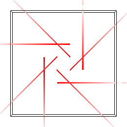
First implement basic animation of the masses. You'll need to compute the spring forces and track the position, velocity, and acceleration of each particle as time progresses. Simple forward/explicit Euler integration is sufficient. You can access the timestep and gravity from the ArgParser class. Initially test your code on the small example shown below and verify that each of the spring forces (structural, shear, and bend/flexion) and the force due to gravity are correct. Pressing 'a' will toggle the animation on and off. Each loop of this continuous animation will call Cloth::Animate() 10 times and then refresh the screen. To take just one step of animation, press the space bar. You can restart the animation from the beginning by pressing 'r'.
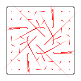
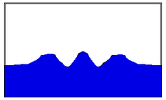
```
simulation -cloth small_cloth.txt -timestep 0.001
```
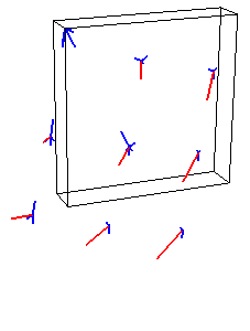
You will need to complete the implementation for the force visualization. Your visualization does not need to match the one above (the blue lines), as long as you find its output informative and helpful in your debugging.
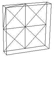
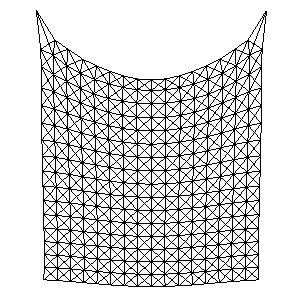
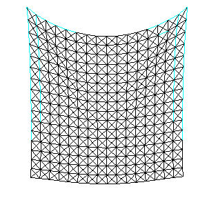
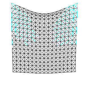
Once your basic spring-mass system is working, test it on the larger example below. As illustrated by Provot, the springs at the corner will stretch too much. Implement the iterative correction/adjustment method for springs that have stretched beyond the specified threshold. The provided code will visualize the "over-stretched" springs in cyan (shown below).
```
simulation -cloth provot_original.txt -timestep 0.001
simulation -cloth provot_correct_structural.txt -timestep 0.001
simulation -cloth provot_correct_structural_and_shear.txt -timestep 0.001
```
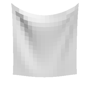
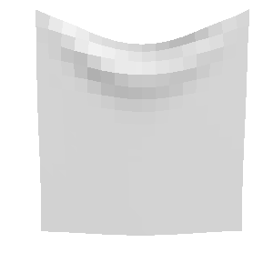
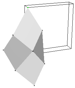
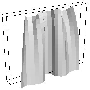
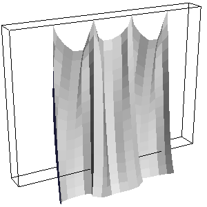
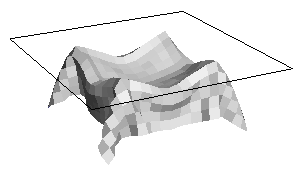
When you are confident that your implementation is complete, test it on the examples below which use different parameter values to mimic different types of cloth. Now experiment with your system and try adjusting the many different parameters. How stable is the simulation? Discuss in your README.txt. Make at least one interesting new test scene. You may extend the input file format as necessary for your new example(s). Describe your new example and how to run it in your README file.
```
simulation -cloth denim_curtain.txt -timestep 0.001
simulation -cloth silk_curtain.txt -timestep 0.001
```
```
simulation -cloth table_cloth.txt -timestep 0.005
```
In your experimentation, you undoubtedly caused the cloth to "explode" at least once. In theory this instability can always be fixed by using a smaller timestep. So now, let's implement an adaptive timestep for the simulator. Start with the timestep provided on the command line, but if the simulation is too stiff (unstable at that timestep), back up, halve the timestep, and try again. What criteria did you use to detect that the system is unstable? Discuss in your README.txt
Now for the second part --- fluid simulation, which is launched like this:
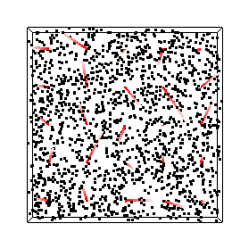
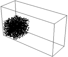
```
  simulation -fluid fluid_random_xy.txt -timestep 0.01
```
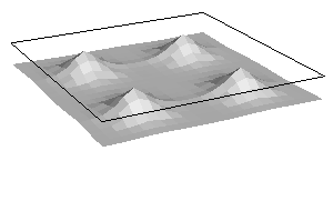
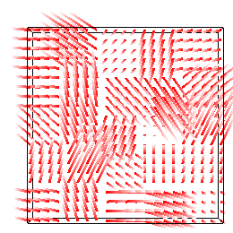
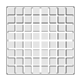
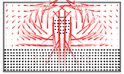
The images below show some visualizations of this dataset of random particles on a 5x5x1 grid. On the left we see the random particles (approximately 64 per cell) and the random initial velocities measured at the center of each cell. Marker particle visualization and velocity visualization are toggled by pressing the 'm' and 'v' keys. Remember that the velocities are actually stored as vectors perpendicular to the face of each cell, visualized by red (x) and green (y) triangles (toggled by pressing the 'e' key). The velocity at the center of each cell is computed by averaging the velocities at the faces on either side of the cell.

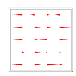
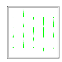
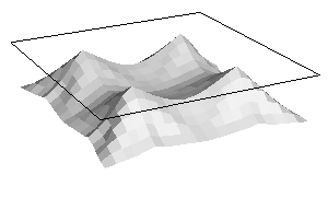
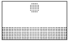
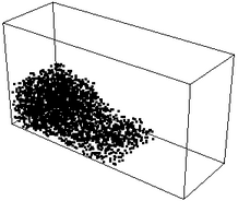
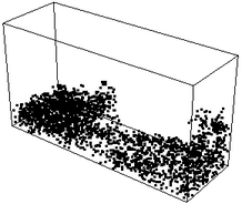
To move particles within the field, we need to compute the velocity at each point within the volume. The simplest thing to do is just use the velocity at the center of the cell for all particles in that cell. The image below left shows this discontinuous velocity field (press 'd' to visualize this "dense" velocity field). Go ahead and press 'a' to animate the particles within this field and you should see why this isn't a good assignment of velocities.

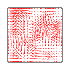
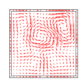
So, your first task is to implement proper velocity interpolation as described in Foster & Metaxas. Once you've carefully implemented the interpolation in the xy plane, run the above simulation again and you should see dense velocity fields like the ones above middle and right. NOTE: In the implementation provided, each cell stores the face velocities (u, v, & w) for the face it shares with the cell in the positive direction along each axis. That is, cell_i,j,k stores u_i+1/2,j,k, v_i,j+1/2,k, and w_i,j,k+1/2. These values are stored in the variables u_plus, v_plus, and w_plus, and the corresponding accessors get_u_plus(), get_v_plus(), and get_w_plus().
To perform 3D fluid simulations your interpolation scheme must correctly account for the z direction as well. Here are 3 test cases to help you verify that your interpolation is working in 3D. The resulting animation should be similar in each of the 3 axis-aligned planes.
```
  simulation -fluid fluid_spiral_xy.txt -timestep 0.01
  simulation -fluid fluid_spiral_yz.txt -timestep 0.01
  simulation -fluid fluid_spiral_zx.txt -timestep 0.01
```
Now let's address the issue of compressibility/incompressibility. You may have noticed that your simulations are a little "bouncy". To emphasize the fact, try this simulation:
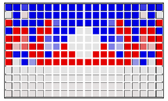
```
  simulation -fluid fluid_compressible.txt -timestep 0.01
```
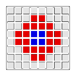
You can press "p" to visualize the pressure in each cell by drawing little cubes for each cell colored by pressure. Initially all the cells are white (pressure == 0). After just a few timesteps a negative pressure (blue) appears in the middle of the grid surrounded by a ring of positive pressure (red). Later in the simulation these values are quite chaotic, introducing noise into the velocity field.

In order to enforce the incompressibility of the flow, you will need to implement the divergence correction originally described by Harlow & Welch and later by Foster & Metaxas. Compute the divergence of each "full" cell and adjust each non-boundary face velocity to absorb its share of excess inflow or outflow. When correctly implemented, the pressure in each cell should be (within epsilon of) zero throughout the simulation and the flow should no longer "bounce".
NOTE: You can swap between compressible and incompressible simulation by editing the following line in the simulation data file and then pressing 'r' to restart the simulation:
```
  flow (in)compressible 
```
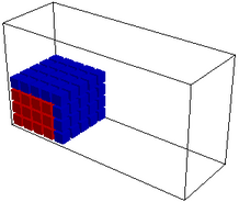
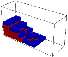
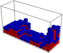
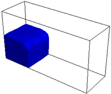
Up to this point, all of the cells in our fluid simulation have been full (had at least one particle). Now let's look at some interesting cases showing the interaction between air and water. Try the examples below. Press "c" to visualize the Marker-And-Cell (MAC) voxels: red == FULL and blue == SURFACE. Press "s" to enable a triangular mesh rendering of the surface using Marching Cubes/Marching Tetras.
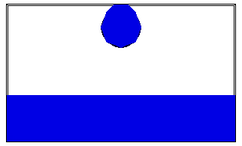
```
  simulation -fluid fluid_drop.txt -timestep 0.01
```
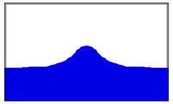
```
  simulation -fluid fluid_dam.txt -timestep 0.01
```
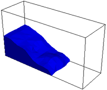
To perform these simulations you will need to extend your incompressibility code to handle surface cells. The divergence of inflow or outflow should be dissipated over the "free" faces of the cell (i.e., faces that this cell shares with EMPTY cells). Note: You can edit the dimensions of your grid by editing the top line of the simulation data file. The "drop" and "dam" shapes will adjust to your new dimensions.
WARNING: Despite spending many hours on the solution implementation, I was not able to sufficiently stabilize these last two examples to match results from the papers we have read. It could be that the timestep was too large (ultimately due to the inherent instability of explicit numerical integration schemes), that the units are not consistent (e.g., grams vs. kilograms), that I've misinterpreted the implementation described in the papers, or that there are bugs in my code. If you are more successful, please let us know :)

Additional References

Harlow & Welch, "Numerical Calculation of Time-Dependent Viscous Incompressible Flow of Fluids with Free Surface," Phys. Fluids, Vol. 8, p. 2182, 1965. (paper copy handed out in lecture).
Practical animation of liquids, Foster & Fedkiw, SIGGRAPH 2001
Visual simulation of smoke, Fedkiw, Stam & Jensen, SIGGRAPH 2001
"Melting and Flowing" Carlson, Mucha, Van Horn III & Turk, ACM SIGGRAPH Symposium on Computer Animation 2002

Ideas for Extra Credit

Include a short paragraph in your README.txt file describing your extensions.

Implement an alternate integration method (Midpoint, Runge-Kutta, implicit Euler, etc.) Compare the performance of each method.
Experiment with the provided Marching Cubes implementation in the fluid simulator. Try different isosurface values (a command line option and keyboard shortcut --- press '+'/'-') and render the isosurfaces of different scalar fields such as density or pressure or divergence (for compressible flows). Discuss in your README.txt file. If you're really motivated, add gouraud shading to the marching cubes surface!
Implement a new visualization/rendering mode (maybe you already did to debug an earlier step).
Create a new fluid test scene (you can create it procedurally, or create a new input file). A fun test scene could include source and sink cells where mass is created and deleted or a spatial- or time-varying force field (instead of a uniform gravity).
Having two physical simulation engines within the same program makes it possible for us to experiment with coupled simulations. Compose a cloth simulation and fluid simulation in the same scene (just load 2 files on the command line). The cloth motion can be driven by the fluid's velocity field, or the fluid motion can be driven by the cloth, or both!

Provided Files (hw2_files.zip)

Basic Code (vectors.h, matrix.h, matrix.cpp, argparser.h, camera.h, camera.cpp, glCanvas.h, glCanvas.cpp, main.cpp, boundingbox.h, boundingbox.cpp, utils.h, Makefile)
Similar to Assignments 1 & 2.
Cloth (cloth.h, cloth.cpp)
A class to store, animate, and paint a 2D grid of masses & springs.
Cloth test scenes (small_cloth.txt, provot_original.txt, provot_correct_structural.txt, provot_correct_structural_and_shear.txt, denim_curtain.txt, silk_curtain.txt, table_cloth.txt)
Fluid (fluid.h, fluid.cpp, cell.h, marching_cubes.h, marching_cubes.cpp)
Fluid test scenes (fluid_random_xy.txt, fluid_spiral_xy.txt, fluid_spiral_yz.txt, fluid_spiral_zx.txt, fluid_compressible.txt, fluid_drop.txt, fluid_dam.txt)

Please read the Homework information page again before submitting.