Advanced Computer Graphics
Contact Information
Office Hours
Syllabus
Prerequisites
Textbook
Grading
Assigned Readings
Calendar
Lecture notes
Lab materials
Homework
Test reviews
Homework
Collaboration Policy
Compilers
gcc/g++ notes
GL/glut notes
Homework Late Policy
Electronic Submission
Assignment 3: Distributed Ray Tracing & Radiosity
The goal of this assignment is to implement two different rendering methods to render two different types of materials: distributed ray tracing for glossy materials and radiosity for diffuse materials. Both rendering systems are implemented as part of an interactive OpenGL viewer similar to previous assignments to help with visualization and debugging. Furthermore since they are implemented in the same system, a hybrid rendering that captures both glossy and diffuse global illumination effects is possible (for extra credit).
Tasks
- First, download and compile the provided files. Press 'r' to
initiate a ray tracing from the current camera position. The image
will appear in the OpenGL window initially as a coarse rendering that
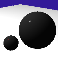
is progressively refined. Your first task is to extend this basic ray
caster to include sphere intersections, shadow rays, and recursive
reflective rays. Poke around in the system to see how the functions
RayTracer::TraceRay, RayTracer::CastRay, and
Face::Intersect are implemented and used. Note that the
OpenGL rendering first converts the spheres to quads, but the original
spheres should be used for ray tracing.
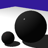
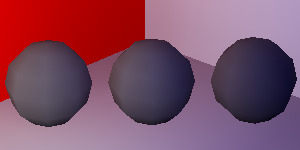
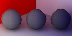
All lights in this system are area light sources (quad patches with
a non-zero emissive color). If only one shadow sample is specified,
simply cast a ray to the center of each area light patch. For
extra credit you may implement soft shadows by casting
multiple rays to points on the area light source. Discuss how
different strategies for selecting the points on the area light source
lead to different performance/quality tradeoffs.
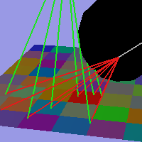
Use the ray tree visualization to debug your recursive rays. When
't' is pressed a ray is traced into the scene through the pixel under
the mouse cursor. The initial ray is drawn in white, reflective rays
are drawn in red, and shadow rays (traced from each intersection to
the lights) are drawn in green. Press 'q' to quit.
./render -size 200 200 -input reflective_spheres.obj -background_color 0.2 0.1 0.6
./render -size 200 200 -input reflective_spheres.obj -background_color 0.2 0.1 0.6 -num_shadow_samples 1
./render -size 200 200 -input reflective_spheres.obj -background_color 0.2 0.1 0.6 -num_shadow_samples 1 -num_bounces 1
./render -size 200 200 -input reflective_spheres.obj -background_color 0.2 0.1 0.6 -num_shadow_samples 10 -num_bounces 3
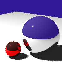

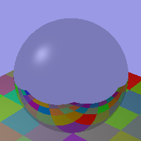
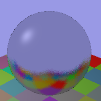
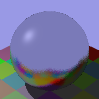
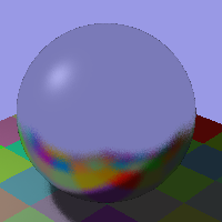
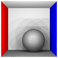
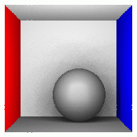
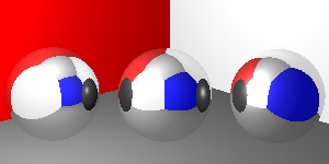
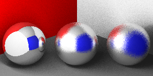
- Next, implement glossy reflections by sampling a cone of rays
around the ideal reflective direction. A "roughness" of 0.0 indicates
a ideal specular reflective surface (all rays reflect in the mirror
directions) and a roughness of 1.0 indicates an ideal diffuse surface
(rays are equally likely to reflect in all directions of the
hemisphere in the "right" side of the surface). If the roughness of a
material is > 0.0 and the number of glossy samples is >
1, then you should sample rays within an appropriately-sized cone
around the ideal reflection direction (make sure you don't sample on
the wrong side of the surface). As the roughness parameter increases,
the fuzziness of the reflections will also increase. Implement
something simple and intuitive initially. For extra credit you may
implement the
Oren-Nayar model (on
Wikipedia).
Try different
values for the number of glossy samples and the roughness (edit the
.obj file). Discuss in your README.txt file how these parameters
affect the quality of the image and the running time.
./render -size 200 200 -input glossy_sphere.obj -background_color 0.6 0.6 0.9 -num_bounces 1
./render -size 200 200 -input glossy_sphere.obj -background_color 0.6 0.6 0.9 -num_bounces 1 -num_glossy_samples 10
./render -size 200 200 -input glossy_sphere.obj -background_color 0.6 0.6 0.9 -num_bounces 1 -num_glossy_samples 10 -num_shadow_samples 1
./render -size 200 200 -input glossy_sphere.obj -background_color 0.6 0.6 0.9 -num_bounces 1 -num_glossy_samples 30 -num_shadow_samples 30
- Next we move on to radiosity. These test scenes are closed,
inward-facing models. Thus, the viewer is configured to cull
(make invisible) "back-facing" polygons (press 'b' to toggle this
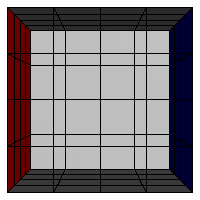
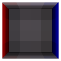
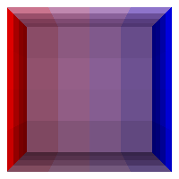
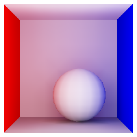
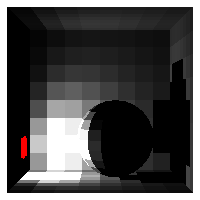
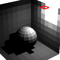
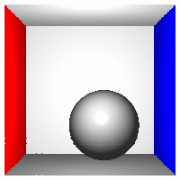
option). Press 'v' to toggle between the different visualization
modes: MATERIALS (a simple shading using the diffuse color of each
material), RADIANCE (the reflected light from each surface),
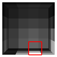
FORM_FACTORS (the patch with the greatest undistributed light is
outlined in red and the relative form factors with every other patch
are displayed in shades of grey), LIGHTS, UNDISTRIBUTED (the light
received by each patch which has not been distributed or absorbed),
and ABSORBED (the light received and absorbed by each patch).
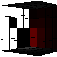
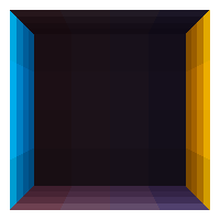
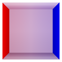
Press 'w' to view the wireframe. The quad mesh model is stored in
a half edge data structure similar to assignment 1. Press 's' to
subdivide the scene. Each quad will be split into 4 quads. Press 'i'
to blend or interpolate the radiosity values. Press 'h' to tone map
the image so your images are similar to the results in the original
radiosity paper. Press the space bar to make one iteration of the
radiosity solver, press 'a' to animate the solver (many iterations),
and press 'c' to reset the radiosity solution. The images below show
various visualizations of the classic Cornell box scene.
./render -size 200 200 -input cornell_box.obj

Your task is to implement the form factor computation and the
radiosity solver. You can choose any method we discussed in class or
read about in various radiosity references. For the Cornell box scene
you do not need to worry about visibility (occlusions). In your
README.txt file, discuss the performance quality tradeoffs between the
number of patches and the complexity of computing a single form
factor.
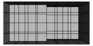
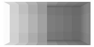
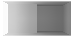
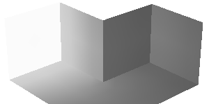
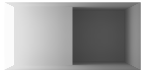
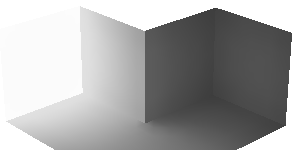
- All non-convex scenes require visibility/occlusion computation
for the form factors. In the simple scene below, light from the left
wall should not reach the deep wall on the right half of the
image. Use the RayTracer::CastRay to incorporate visibility
into the form factor computation when the number of shadow rays is
> 0. The last two images show the scene with visibility correctly
accounted for. Comment on the order notation of the brute force
algorithm in your README.txt file. For extra credit, implement and
analyze a more efficient method.
./render -size 300 150 -input l.obj
./render -size 300 150 -input l.obj -num_form_factor_samples 100
./render -size 300 150 -input l.obj -num_shadow_samples 1
./render -size 300 150 -input l.obj -num_form_factor_samples 10 -num_shadow_samples 1
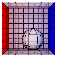
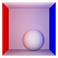
Here is another test scene that requires visibility in the form
factor computation:
./render -size 200 200 -input cornell_box_diffuse_sphere.obj
./render -size 200 200 -input cornell_box_diffuse_sphere.obj -sphere_rasterization 16 12
./render -size 200 200 -input cornell_box_diffuse_sphere.obj -num_shadow_samples 1
./render -size 200 200 -input cornell_box_diffuse_sphere.obj -num_shadow_samples 1 -sphere_rasterization 16 12
- Finally, for extra credit integrate the global illumination
data computed using radiosity with the reflections and high frequency
shadows from ray tracing. Note how neither method alone is able to
produce a satisfactory rendering of the scene below:
./render -size 300 150 -input cornell_box_reflective_spheres.obj -num_bounces 1
./render -size 300 150 -input cornell_box_reflective_spheres.obj -num_bounces 1 -num_glossy_samples 10
./render -size 300 150 -input cornell_box_reflective_spheres.obj -num_bounces 3 -num_shadow_samples 100 -num_glossy_samples 10

Other Ideas for Extra Credit
Include a short paragraph in your README.txt file describing
your extensions.
- Implement a "smart" subdivision scheme to refine the mesh in
areas with a high radiance gradient.
- Implement progressive radiosity with the ambient term.
- Compute the penumbra and umbra regions of an area light source
for discontinuity meshing, etc.
- Create an interesting new test scene or visualization.
- Render directly to a file to speed up the rendering process
(pixel-by-pixel OpenGL rendering is slow).
- Improve the performance of either rendering system. Analyze
the order notation of the operations before and after your
improvements and the running times.
- Implement other recursive ray tracing or distributed ray
tracing effects. Include sample command lines to demonstrate your new
features. Include sample images (since we will not have time for long
runs while grading).
Provided Files (hw3_files.zip)
- Basic Code (argparser.h, bag.h, boundingbox.h, boundingbox.cpp,
camera.h, camera.cpp, glCanvas.h, glCanvas.cpp, main.cpp, matrix.h,
matrix.cpp, utils.h, vectors.h, Makefile)
Similar to the previous assignments.
- Half-Edge Quad Mesh Data Structure (edge.h,
edge.cpp,
face.h,
face.cpp,
mesh.h,
mesh.cpp,
sphere.h,
sphere.cpp,
material.h,
material.cpp,
vertex.h,
vertex_parent.h)
Similar to the triangle half-edge data structure you implemented in
assignment 1. Spheres are stored both in center/radius format and
converted to quad patches for use with radiosity.
- Raytracing & Radiosity (raytracer.cpp, raytracer.h, ray.h,
hit.h, raytree.h, raytree.cpp, radiosity.h, radiosity.cpp)
The basic rendering engines and visualization tools.
- Test scenes (reflective_spheres.obj, glossy_sphere.obj,
cornell_box.obj, l.obj, cornell_box_diffuse_sphere.obj, cornell_box_reflective_spheres.obj)
Note: These test data sets are a non-standard extension of
the .obj file format. Feel free to modify the files as you wish to
implement extensions for extra credit.
Please read the Homework information page again before submitting.
All lights in this system are area light sources (quad patches with a non-zero emissive color). If only one shadow sample is specified, simply cast a ray to the center of each area light patch. For extra credit you may implement soft shadows by casting multiple rays to points on the area light source. Discuss how different strategies for selecting the points on the area light source lead to different performance/quality tradeoffs.
Use the ray tree visualization to debug your recursive rays. When
't' is pressed a ray is traced into the scene through the pixel under
the mouse cursor. The initial ray is drawn in white, reflective rays
are drawn in red, and shadow rays (traced from each intersection to
the lights) are drawn in green. Press 'q' to quit.
./render -size 200 200 -input reflective_spheres.obj -background_color 0.2 0.1 0.6
./render -size 200 200 -input reflective_spheres.obj -background_color 0.2 0.1 0.6 -num_shadow_samples 1
./render -size 200 200 -input reflective_spheres.obj -background_color 0.2 0.1 0.6 -num_shadow_samples 1 -num_bounces 1
./render -size 200 200 -input reflective_spheres.obj -background_color 0.2 0.1 0.6 -num_shadow_samples 10 -num_bounces 3
./render -size 200 200 -input glossy_sphere.obj -background_color 0.6 0.6 0.9 -num_bounces 1 ./render -size 200 200 -input glossy_sphere.obj -background_color 0.6 0.6 0.9 -num_bounces 1 -num_glossy_samples 10 ./render -size 200 200 -input glossy_sphere.obj -background_color 0.6 0.6 0.9 -num_bounces 1 -num_glossy_samples 10 -num_shadow_samples 1 ./render -size 200 200 -input glossy_sphere.obj -background_color 0.6 0.6 0.9 -num_bounces 1 -num_glossy_samples 30 -num_shadow_samples 30
Press 'w' to view the wireframe. The quad mesh model is stored in
a half edge data structure similar to assignment 1. Press 's' to
subdivide the scene. Each quad will be split into 4 quads. Press 'i'
to blend or interpolate the radiosity values. Press 'h' to tone map
the image so your images are similar to the results in the original
radiosity paper. Press the space bar to make one iteration of the
radiosity solver, press 'a' to animate the solver (many iterations),
and press 'c' to reset the radiosity solution. The images below show
various visualizations of the classic Cornell box scene.
./render -size 200 200 -input cornell_box.obj
Your task is to implement the form factor computation and the radiosity solver. You can choose any method we discussed in class or read about in various radiosity references. For the Cornell box scene you do not need to worry about visibility (occlusions). In your README.txt file, discuss the performance quality tradeoffs between the number of patches and the complexity of computing a single form factor.
./render -size 300 150 -input l.obj ./render -size 300 150 -input l.obj -num_form_factor_samples 100 ./render -size 300 150 -input l.obj -num_shadow_samples 1 ./render -size 300 150 -input l.obj -num_form_factor_samples 10 -num_shadow_samples 1
Here is another test scene that requires visibility in the form
factor computation:
./render -size 200 200 -input cornell_box_diffuse_sphere.obj
./render -size 200 200 -input cornell_box_diffuse_sphere.obj -sphere_rasterization 16 12
./render -size 200 200 -input cornell_box_diffuse_sphere.obj -num_shadow_samples 1
./render -size 200 200 -input cornell_box_diffuse_sphere.obj -num_shadow_samples 1 -sphere_rasterization 16 12
./render -size 300 150 -input cornell_box_reflective_spheres.obj -num_bounces 1 ./render -size 300 150 -input cornell_box_reflective_spheres.obj -num_bounces 1 -num_glossy_samples 10 ./render -size 300 150 -input cornell_box_reflective_spheres.obj -num_bounces 3 -num_shadow_samples 100 -num_glossy_samples 10
Similar to the previous assignments.
Similar to the triangle half-edge data structure you implemented in assignment 1. Spheres are stored both in center/radius format and converted to quad patches for use with radiosity.
The basic rendering engines and visualization tools.
Note: These test data sets are a non-standard extension of the .obj file format. Feel free to modify the files as you wish to implement extensions for extra credit.