Query Optimization#

Given a query written in logic, we would like to find out how to execute it as fast as possible, by taking into account:
- how the data is stored
- which query operations are involved and their various implementations
Query optimization is one of the most complex tasks provided by the database, often one of the main reasons to use a database system for complex queries.
- Releaves the user from the burden to think about implementation and concentrate on logic (though you should really not write horrible queries)
We will only give an overview of different steps, but the exact details are much more complex.

Overview#

Query optimization is the process of taking a query written in SQL and converting to a query implementation plan.
A query implementation plan is a query tree with:
- database tables are leaf nodes,
- each internal node is a query operator with an assignment of a specific implementation and memory allocation,
- and the root of the node is a correct implementation of the given query.
Query optimization involves many different steps:
- Parse the query and rewrite if needed (for example eliminate nested correlated subexpressions if possible, simplify boolean expressions, etc.)
- Create a preliminary query tree
- Find access paths for selections (different indices that might apply)
  
  Includes also potential sort operations if it can help the query for one or more operators
- Find different ways to join relations (which access paths to use and the join ordering) by enumerating all possible choices
  
  Choose the lowest cost method by estimating the cost of each different option and eliminating options that cannot outpeform others
Next, we will see each step.

Query Parsing and Rewriting#

First, parsing checks to see queries are valid with respect to the table and attribute names, data types.
Take view names and replace them with their definitions.
Rewrite queries to simplify boolean expressions and resolve subexpressions that are always true or false.
```
SELECT A FROM R WHERE R.A > 5 AND R.A < 4;
```
returns nothing (the condition can never be true).
```
SELECT A FROM R WHERE R.B >= R.C OR R.C >= R.B;
```
equivalent to a simpler query:
```
SELECT A FROM R;
```
More complex rewritings require semantic processing of the queries and schema.

Especially, try to rewrite nested queries without nesting if possible.
```
SELECT
   r.a
   , r.b
FROM
   r
WHERE
   r.a IN (SELECT s.a FROM s)
```
rewrite as:
```
SELECT
    r.a
    , r.b
FROM
    r
    ,s
WHERE
    r.a=s.a
```
but be careful about semantic equivalences. Are these two always equivalent?

Suppose we are given:

SELECT
   dept.name
FROM
   dept
WHERE
   dept.num-of-machines >=
       (SELECT count(emp.*) FROM emp
        WHERE dept.name = emp.deptname)

Is this equivalent to?

SELECT
   dept.name
FROM
   dept
   , emp
WHERE
   dept.name = emp.dept-name
GROUP BY
   dept.name, dept.num-of-machines
HAVING
   dept.num-of-machines >= count(emp.*)

Query Trees#

An SQL query is translated to an equivalent query tree.
A query treee has
- Tables in the query as leaf nodes
- Relational algebra operators as nodes
- The root of the tree returns the correct results for the given query.
A single query can have many equivalent query trees due to the properties of the relational algebra operators.
The query optimizer will consider all potential query trees when deciding how to optimize the query.

Query Rewriting Rules (Algebraic Equivalences)#

Suppose we are given R(A,B,C) and S(D,E,F).

Selections#

Selections can be pushed through joins and Cartesian products.

\[ \sigma_{A=5 \mbox{ and } C>20} (R\,\bowtie_{C=D}\,S) = (\sigma_{A=5 \mbox{ and } C>20}\, R) \,\bowtie_{C=D}\, (\sigma_{D>20}\,S) \]

Note that the selection over R also results in a selection over S.
The reverse is also true:

\[ (\sigma_{B=5}\, R) \,\bowtie_{C=D}\, S = \sigma_{B=5}\, (R\,\bowtie{C=D}\, S) \]

First, push all selections high up the tree and push them all the way down.
Note that selections open up different access paths to the relation (i.e. indices) and can significantly reduce the size of joins.
There are cases in which applying some selections early may not be desirable. We will use cost to guide when to do this.
Selections can be joined with Cartesian products for a join condition:

\[ \sigma_{C=D} (R\,\times\,S) = R\,\bowtie_{C=D}\, S \]

Projections#

Projections can be pushed through joins, Cartesian products to reduce the size of the output

\[ \Pi_{B,E} (R\,\bowtie_{C=D}\,S) = \Pi_{B,E} ((\Pi_{B,C}\, R) \,\bowtie\, (\Pi_{D,E}\, S)) \]

Simply remove attributes not needed in higher level nodes at each step.

Even though the number of tuples do not change (bag projection), the length of each tuple is smaller and more tuples can fit in a single memory block.

Joins#

Joins are associative and commutative (they can be shuffled).

\[ \begin{align}\begin{aligned} R \bowtie S = S \bowtie R\\ R \bowtie (S \bowtie T) = (R \bowtie S) \bowtie T \end{aligned}\end{align} \]

We will see join ordering is a crucial part of query optimization shortly.

Cost-based Query Optimization#

Given alternate query trees, find the lowest cost one.
We do not really need to generate all possible query trees, but find:
- All potential access paths for selections (indices and table scans)
- Join orderings that combine these access paths with specific join implementations
- Estimate the cost of a partial query plan and eliminate other plans that can never be cheaper.
To be able to estimate the cost of query plans, we need to know:
- Cardinality estimation: How many tuples we expect as the output of joins and selections
- Space estimation: The size of the tuples on disk to estimate how many disk pages are needed to store them.
  
  Space estimation is easy due to the knowledge of schema. We will disregard this for now.

Cost-Based Query Optimization#

Generate and estimate the cost of different access paths to base relations (with or without using different indices)
Consider sorting as an option, even though it is an upfront cost, it might help other operations up the query tree.
Incorporate projections when possible to reduce size of the tuples and other methods to reduce size of relations that can be done on the fly:

On the fly operations do not require additional cost. They apply to tuples as they are produced in memory.

Evaluate all possible ways to combine these relations by considering join orderings using dynamic programming:

Consider all two way join orderings to construct a partial query tree
Estimate the cost so far

While there are joins to add:
    Consider adding a new join to a partial query tree
    and estimate cost

    Remove all query trees with fewer joins that are costlier
    (because adding a join will only increase the cost)
    with the exception of trees involving sorts (their benefit
    may show later)

Join orderings#

Considering all possible join orderings may be too costly.

For a three relation join, there are many options:

(R join S) join T        R join (S join T)
(S join R) join T        S join (R join T)
(T join S) join R        T join (S join R)
(S join T) join R        S join (T join R)
(R join T) join S        R join (T join S)
(T join R) join S        T join (R join S)

We need to decide on the shape of join tree, the ordering of the joins and then decide inner/outer relations for each join.
Main join tree types:
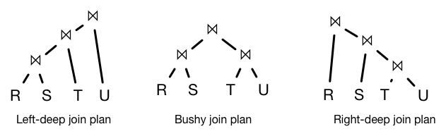
- Left-deep joins are particularly useful because the output of one operation can be pipelined into the next join operation
- Bushy joins can be very useful when relations are stored in different disks or machines, allowing the database to use parallelism in computing the query.
  
  In cases where relations are remote, other operations are introduced such as semi-joins, that filter for key values that will participate in joins before shipping data across a network.
In this class, we will assume only left-deep join trees with pipelined operations.

The relation ordering (inner/outer) is determined by the underlying join operation. Often it is beneficial to put smaller relation as the outer relation, reducing the number of passes over the inner relation.

Join ordering example#

Suppose we have the following statistics for the following query:
```
SELECT R.E,S.F,T.G FROM R,S,T WHERE R.A=S.B AND S.C=T.D
```
RELATION

TUPLES

PAGES

R

10,000

500

S

200,000

1,000

T

50,000

2,000

ATTR

N_DISTINCT

R.A

10,000

S.B

9,000

S.C

500

T.D

800

RELATION	TUPLES	PAGES
R	10,000	500
S	200,000	1,000
T	50,000	2,000

ATTR	N_DISTINCT
R.A	10,000
S.B	9,000
S.C	500
T.D	800

Let’s disregard the size reduction that can be obtained through projections. Assume that after a join, we can fit about 50 tuples per page.

We will only consider block nested loop joins. Assume each operation has M=101 pages.

exp(R join S) = 10,000*200,000/10,000 = 200,000 (tuples fits in 2,000 pages)

Block-nested loop join: 500 + 5*1,000 = 5,500 pages

exp(S join T) = 200,000*50,000/800= 12,500,000 tuples (fits in 250,000 pages)

Block-nested loop join: 1,000 + 10*2,000 = 21,000 pages

exp(R join T) = 10,000*50,000 = 500,000,000 tuples (fits in 10,000,000 pagees)

Note that this is a Cartesian product as there are no join conditions
between R and T.

Block-nested loop join: 500 + 5*2,000 = 10,500 pages

Now, we will see how to add a third join. Let’s start with the cheapest operation and go forward.

exp( (R join S) join T ) = 200,000*50,000/800= 100000000/8 =
12,500,000 tuples (note: this is the same for all the different
plans, so we will not compute this for the rest.)


Read R join S into 100 pages, and read T into the remaining.

T is read: 2,000/100 = 20 times (size of R join S fits in 2,000 pages)

No additional cost to read R join S, the tuples are in memory as
it is being pipelined from the operator below:

Total cost = (Cost of R join S) + (Cost of reading T 20 times for the last join)
Total cost = 5,500 + 20*2,000 = 45,500 pages

Let’s see the same for other joins:

Cost of (S join T) join R = 21000 + 2500*500 = 1,271,000

Cost of (R join T) join S = 10500 + 100000*1000 = 100,010,500

The best plan is: (R join S) join T

Query Optimization

Contents