Advanced Computer Graphics
Contact Information
Office Hours
Syllabus
Prerequisites
Textbook
Grading
Assigned Readings
Calendar
Lecture notes
Lab materials
Homework
Test reviews
Homework
Collaboration Policy
Compilers
gcc/g++ notes
GL/glut notes
Homework Late Policy
Electronic Submission
Final Project
Spring '11 Projects
Spring '10 Projects
Spring '09 Projects
Spring '08 Projects
Spring '07 Projects
Assignment 3: Ray Tracing, Radiosity, & Photon Mapping
The goal of this assignment is to implement pieces of three different rendering methods that can be used to capture important rendering effects including reflection, color bleeding, and caustics. These different rendering methods are implemented within a single interactive OpenGL viewer similar to previous assignments to help with visualization and debugging. Furthermore, since they are implemented in the same system, hybrid renderings that capture combinations are possible.
Tasks
- First, download and compile the provided files. Run the program
using the sample command lines below. Press 'r' to initiate a ray
tracing from the current camera position. The image will appear in
the OpenGL window initially as a coarse rendering that is
progressively refined. (When you use the mouse to change the camera
position, the raytracing will be canceled and you will be returned to
the basic OpenGL rendering of the scene.) Press 'q' to quit.
Initially, you will only see the ground plane -- that's because the
sphere intersection routine has not been implemented! This is your
first task. You'll have to do a little work beyond our discussion in
class to handle spheres that are not centered at the origin. Note
that our OpenGL rendering first converts the spheres to quads, but the
original spheres should be used for ray tracing intersection.
- Your next task is to extend this basic ray caster to include
shadow rays and recursive reflective rays. Continue to poke around in
the system to see how the RayTracer::TraceRay and
RayTracer::CastRay functions are implemented and used. Note
that all lights in this system are area light sources (quad patches
with a non-zero emissive color). If only one shadow sample is
specified, simply cast a ray to the center of each area light patch.
Use the ray tree visualization to debug your recursive rays. When
't' is pressed, a ray is traced into the scene through the pixel under
the mouse cursor. You will have to add calls to
RayTree::AddShadowSegment and
RayTree::AddReflectiveSegment in your recursive raytracing
code. The initial main/camera/eye ray is drawn in white, reflective
rays are drawn in red, and shadow rays (traced from each intersection
to the lights) are drawn in green.
./render -input reflective_spheres.obj
./render -input reflective_spheres.obj -num_bounces 1
./render -input reflective_spheres.obj -num_bounces 3 -num_shadow_samples 1


- Next, let's implement a couple of the features of distribution
ray tracing: soft shadows and antialiasing. For soft shadows you
will cast multiple shadow rays to a random selection of points on the
light source. For antialiasing, you will cast multiple rays from the
eye through the pixel on the image plane. In your README.txt discuss
how you generated those random points (on the light source and within
the pixel).
For extra credit, you can implement different strategies for
selecting these random points (e.g., stratified sampling or jittered
samples) and discuss in your README.txt the performance/quality
tradeoffs. Also, for extra credit you can implement other effects
using distribution ray tracing such as glossy surfaces, motion blur,
or depth of field.
./render -input textured_plane_reflective_sphere.obj -num_bounces 1 -num_shadow_samples 1
./render -input textured_plane_reflective_sphere.obj -num_bounces 1 -num_shadow_samples 4
./render -input textured_plane_reflective_sphere.obj -num_bounces 1 -num_shadow_samples 9 -num_antialias_samples 9


- Next we move on to radiosity. These test scenes are closed,
inward-facing models. Thus, the viewer is configured to cull
(make invisible) "back-facing" polygons (press 'b' to toggle this
option). Press 'v' to toggle between the different visualization
modes: MATERIALS (the default simple shading using the diffuse color
of each material), RADIANCE (the reflected light from each surface),
FORM_FACTORS (the patch with the greatest undistributed light is
outlined in red and the relative form factors with every other patch
are displayed in shades of grey), LIGHTS, UNDISTRIBUTED (the light
received by each patch which has not been distributed or absorbed),
and ABSORBED (the light received and absorbed by each patch).
Press 'w' to view the wireframe. The quad mesh model is stored in
a half edge data structure similar to assignment 1. Press 's' to
subdivide the scene. Each quad will be split into 4 quads. Press 'i'
to blend or interpolate the radiosity values. Press the space bar to
make one iteration of the radiosity solver, press 'a' to animate the
solver (many iterations), and press 'c' to reset the radiosity
solution. The images below show various visualizations of the classic
Cornell box scene.
./render -input cornell_box.obj


The top row of images shows: the MATERIALS, with wireframe after 2
subdivisions, the RADIANCE after allowing the top 16 patches to shoot
their light in the scene, the RADIANCE after many iterations (near
convergence), and the smooth interpolation of those values. The
bottom row shows: the FORM FACTORS from a patch on the left wall
(outlined in red) to all other patches in the scene, the ABSORBED
light after light shooting from the top 16 patches, and ABSORBED light
after many iterations, and a visualization of the UNDISTRIBUTED light
after the top 5 patches have shot their light into the scene.
Your task is to implement the form factor computation and the
radiosity solver. You can choose any method we discussed in class or
read about in various radiosity references. For the Cornell box scene
you do not need to worry about visibility (occlusions). In your
README.txt file, discuss the performance quality tradeoffs between the
number of patches and the complexity of computing a single form
factor.
- All non-convex scenes require visibility/occlusion computation
for the form factors. In the simple scene below, light from the left
wall should not reach the deep wall on the right half of the
image. Use the RayTracer::CastRay to incorporate visibility
into the form factor computation when the number of shadow rays is
> 0. The last two images show the scene with visibility correctly
accounted for. Comment on the order notation of the brute force
algorithm in your README.txt file. Note that the mesh stores both the
subdivided quads and the original quads. Checking for
occlusion with the original quads will improve the running time. For
extra credit, implement additional accelerations for the visibility
computation.
./render -size 300 150 -input l.obj
./render -size 300 150 -input l.obj -num_form_factor_samples 100
./render -size 300 150 -input l.obj -num_shadow_samples 1
./render -size 300 150 -input l.obj -num_form_factor_samples 10 -num_shadow_samples 1


Here is another test scene that requires visibility in the form
factor computation:
./render -input cornell_box_diffuse_sphere.obj -sphere_rasterization 16 12
./render -input cornell_box_diffuse_sphere.obj -sphere_rasterization 16 12 -num_shadow_samples 1


The same scene rendered using ray tracing is too dark. Even when
we approximate global illumination using an ambient term, the scene is
missing the characteristic color bleeding.
./render -input cornell_box_diffuse_sphere.obj -ambient_light 0.0 0.0 0.0
./render -input cornell_box_diffuse_sphere.obj -ambient_light 0.0 0.0 0.0 -num_shadow_samples 1
./render -input cornell_box_diffuse_sphere.obj -ambient_light 0.2 0.2 0.2 -num_shadow_samples 1
./render -input cornell_box_diffuse_sphere.obj -ambient_light 0.2 0.2 0.2 -num_shadow_samples 10
./render -input cornell_box_diffuse_sphere.obj -ambient_light 0.2 0.2 0.2 -num_shadow_samples 100


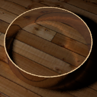
- The third piece of this homework assignment is to use photon
mapping to capture caustics -- the concentration of light due to
specular reflection (or similarly, by refraction). Our primary
example will be the heart-shaped caustic created when light is
reflected off the interior of a shiny cylindrical metal ring.
The first step is to trace photons into the scene. Press 'p' to
call your code which will trace the specified number of photons
throughout the scene. When a photon hits a surface, the photon's
energy and incoming direction are recorded. Depending on the material
properties of the surface, the photon will be recursively traced in
the mirror direction (for reflective materials) or a random direction
(for diffuse materials) or terminated. Don't forget to multiply by
the diffuse or reflective colors to decrease the energy of the photon
appropriately. How do you decide when to stop bouncing the photons?
A visualization of the photon hits is provided in the
PhotonMapping class (shown below left). Press 'l' to toggle the
rendering of the photons. A KD-tree spatial data structure is also
provided to store the photons where they hit, which will allow you to
quickly collect all points within a query boundary box. Press 'k' to
toggle the rendering of the kdtree wireframe visualization.
The second step is to extend your ray tracing implementation to
search for the k closest photons to the hit point. The
energy and incoming direction of each photon is accumulated (according
the the surface reflectance properties) to determine how much
additional light is reflected to the camera (added to the raytracing
result instead of the traditional "ambient" lighting hack). To
trigger raytracing with photon gathering, press 'g'. The third image
below is a traditional recursive raytracing of the scene. The
rightmost image adds in the energy from the photon map to capture the
heart-shaped caustic.
./render -input reflective_ring.obj -num_photons_to_shoot 10000 -num_bounces 2 -num_shadow_samples 10
./render -input reflective_ring.obj -num_photons_to_shoot 500000 -num_bounces 2 -num_shadow_samples 10 -num_antialias_samples 4


- Photon mapping can also enable the raytracer to capture
diffuse global illumination effects such as color bleeding. However,
a large number of photons is required to capture these subtle effects
without significant noise or "splotchy" artifacts. Note: Extending
the basic mechanism of photon mapping with irradiance caching will
greatly improve the performance (which would certainly be worth extra
credit!).
./render -input cornell_box_diffuse_sphere.obj -num_photons_to_shoot 500000 -num_shadow_samples 500 -num_photons_to_collect 500
./render -input cornell_box_reflective_sphere.obj -num_photons_to_shoot 500000 -num_shadow_samples 500 -num_photons_to_collect 500 -num_bounces 1


Other Ideas for Extra Credit
Include a short paragraph in your README.txt file describing
your extensions.
- Implement refraction or glossy reflections for traditional
recursive ray tracing.
- Implement a "smart" subdivision scheme for radiosity to refine
the mesh in areas with a high radiance gradient.
- Implement progressive radiosity with an ambient term to render
the undistributed illumination. This rendering is particularly useful
when paired with incremental form factor computation.
- Compute the penumbra and umbra regions of an area light source
for discontinuity meshing in radiosity, etc.
- Save the raytracing results directly to a file to speed up the
rendering process (the interactive pixel-by-pixel OpenGL rendering is
useful for debugging, but quite slow). A simple image class is
included with the provided files.
- Improve the performance of the rendering system. Use a code
profiling tool and/or analyze the order notation of the algorithms
before and after your improvements and the running times. Document
your findings in your README.tx file.
- Implement irradiance caching with your photon mapping code.
- Implement refraction in your photon tracing code to render
caustics from transparent objects.
- Create an interesting new test scene or visualization.
- Implement other recursive ray tracing or distributed ray
tracing effects. Include sample command lines to demonstrate your new
features.
Include sample images with your submission (since we will
not have time for long runs while grading).
Provided Files (hw3_files.zip)
- Basic Code (argparser.h, boundingbox.h, camera.h, camera.cpp,
glCanvas.h, glCanvas.cpp, main.cpp, matrix.h, matrix.cpp, utils.h,
vectors.h, MersenneTwister.h, Makefile)
Similar to the previous assignments. NOTE: MersenneTwister is a
high quality pseudo-random number generator. Like drand48/srand48, it
can be seeded with a constant to provide repeatable sequences for
deterministic behavior while debugging.
- Half-Edge Quad Mesh Data Structure (edge.h,
edge.cpp,
hash.h,
face.h,
face.cpp,
mesh.h,
mesh.cpp,
primitive.h,
sphere.h,
sphere.cpp,
cylinder_ring.h,
cylinder_ring.cpp,
material.h,
material.cpp,
vertex.h)
Similar to the triangle half-edge data structure you implemented in
assignment 1. Spheres are stored both in center/radius format and
converted to quad patches for use with radiosity.
- Raytracing, Radiosity, & Photon Mapping (raytracer.cpp,
raytracer.h, ray.h, hit.h, raytree.h, raytree.cpp, radiosity.h,
radiosity.cpp, photon_mapping.h, photon_mapping.cpp, image.h,
image.cpp, photon.h, kdtree.cpp, kdtree.h)
The basic rendering engines and visualization tools and image class for loading and saving .ppm files.
- Test scenes (reflective_spheres.obj,
textured_plane_reflective_sphere.obj,
green_mosaic.ppm,
cornell_box.obj,
l.obj,
cornell_box_diffuse_sphere.obj,
reflective_ring.obj,
wood.ppm,
cornell_box_reflective_sphere.obj)
Note: These test data sets are a non-standard extension of
the .obj file format. Feel free to modify the files as you wish to
implement extensions for extra credit.
Please read the Homework information page again before submitting.
Initially, you will only see the ground plane -- that's because the sphere intersection routine has not been implemented! This is your first task. You'll have to do a little work beyond our discussion in class to handle spheres that are not centered at the origin. Note that our OpenGL rendering first converts the spheres to quads, but the original spheres should be used for ray tracing intersection.
Use the ray tree visualization to debug your recursive rays. When
't' is pressed, a ray is traced into the scene through the pixel under
the mouse cursor. You will have to add calls to
RayTree::AddShadowSegment and
RayTree::AddReflectiveSegment in your recursive raytracing
code. The initial main/camera/eye ray is drawn in white, reflective
rays are drawn in red, and shadow rays (traced from each intersection
to the lights) are drawn in green.
./render -input reflective_spheres.obj
./render -input reflective_spheres.obj -num_bounces 1
./render -input reflective_spheres.obj -num_bounces 3 -num_shadow_samples 1
For extra credit, you can implement different strategies for
selecting these random points (e.g., stratified sampling or jittered
samples) and discuss in your README.txt the performance/quality
tradeoffs. Also, for extra credit you can implement other effects
using distribution ray tracing such as glossy surfaces, motion blur,
or depth of field.
./render -input textured_plane_reflective_sphere.obj -num_bounces 1 -num_shadow_samples 1
./render -input textured_plane_reflective_sphere.obj -num_bounces 1 -num_shadow_samples 4
./render -input textured_plane_reflective_sphere.obj -num_bounces 1 -num_shadow_samples 9 -num_antialias_samples 9
Press 'w' to view the wireframe. The quad mesh model is stored in
a half edge data structure similar to assignment 1. Press 's' to
subdivide the scene. Each quad will be split into 4 quads. Press 'i'
to blend or interpolate the radiosity values. Press the space bar to
make one iteration of the radiosity solver, press 'a' to animate the
solver (many iterations), and press 'c' to reset the radiosity
solution. The images below show various visualizations of the classic
Cornell box scene.
./render -input cornell_box.obj
The top row of images shows: the MATERIALS, with wireframe after 2 subdivisions, the RADIANCE after allowing the top 16 patches to shoot their light in the scene, the RADIANCE after many iterations (near convergence), and the smooth interpolation of those values. The bottom row shows: the FORM FACTORS from a patch on the left wall (outlined in red) to all other patches in the scene, the ABSORBED light after light shooting from the top 16 patches, and ABSORBED light after many iterations, and a visualization of the UNDISTRIBUTED light after the top 5 patches have shot their light into the scene.
Your task is to implement the form factor computation and the radiosity solver. You can choose any method we discussed in class or read about in various radiosity references. For the Cornell box scene you do not need to worry about visibility (occlusions). In your README.txt file, discuss the performance quality tradeoffs between the number of patches and the complexity of computing a single form factor.
./render -size 300 150 -input l.obj ./render -size 300 150 -input l.obj -num_form_factor_samples 100 ./render -size 300 150 -input l.obj -num_shadow_samples 1 ./render -size 300 150 -input l.obj -num_form_factor_samples 10 -num_shadow_samples 1
Here is another test scene that requires visibility in the form
factor computation:
./render -input cornell_box_diffuse_sphere.obj -sphere_rasterization 16 12
./render -input cornell_box_diffuse_sphere.obj -sphere_rasterization 16 12 -num_shadow_samples 1
The same scene rendered using ray tracing is too dark. Even when
we approximate global illumination using an ambient term, the scene is
missing the characteristic color bleeding.
./render -input cornell_box_diffuse_sphere.obj -ambient_light 0.0 0.0 0.0
./render -input cornell_box_diffuse_sphere.obj -ambient_light 0.0 0.0 0.0 -num_shadow_samples 1
./render -input cornell_box_diffuse_sphere.obj -ambient_light 0.2 0.2 0.2 -num_shadow_samples 1
./render -input cornell_box_diffuse_sphere.obj -ambient_light 0.2 0.2 0.2 -num_shadow_samples 10
./render -input cornell_box_diffuse_sphere.obj -ambient_light 0.2 0.2 0.2 -num_shadow_samples 100
The first step is to trace photons into the scene. Press 'p' to call your code which will trace the specified number of photons throughout the scene. When a photon hits a surface, the photon's energy and incoming direction are recorded. Depending on the material properties of the surface, the photon will be recursively traced in the mirror direction (for reflective materials) or a random direction (for diffuse materials) or terminated. Don't forget to multiply by the diffuse or reflective colors to decrease the energy of the photon appropriately. How do you decide when to stop bouncing the photons?
A visualization of the photon hits is provided in the PhotonMapping class (shown below left). Press 'l' to toggle the rendering of the photons. A KD-tree spatial data structure is also provided to store the photons where they hit, which will allow you to quickly collect all points within a query boundary box. Press 'k' to toggle the rendering of the kdtree wireframe visualization.
The second step is to extend your ray tracing implementation to
search for the k closest photons to the hit point. The
energy and incoming direction of each photon is accumulated (according
the the surface reflectance properties) to determine how much
additional light is reflected to the camera (added to the raytracing
result instead of the traditional "ambient" lighting hack). To
trigger raytracing with photon gathering, press 'g'. The third image
below is a traditional recursive raytracing of the scene. The
rightmost image adds in the energy from the photon map to capture the
heart-shaped caustic.
./render -input reflective_ring.obj -num_photons_to_shoot 10000 -num_bounces 2 -num_shadow_samples 10
./render -input reflective_ring.obj -num_photons_to_shoot 500000 -num_bounces 2 -num_shadow_samples 10 -num_antialias_samples 4
./render -input cornell_box_diffuse_sphere.obj -num_photons_to_shoot 500000 -num_shadow_samples 500 -num_photons_to_collect 500 ./render -input cornell_box_reflective_sphere.obj -num_photons_to_shoot 500000 -num_shadow_samples 500 -num_photons_to_collect 500 -num_bounces 1
Similar to the previous assignments. NOTE: MersenneTwister is a high quality pseudo-random number generator. Like drand48/srand48, it can be seeded with a constant to provide repeatable sequences for deterministic behavior while debugging.
Similar to the triangle half-edge data structure you implemented in assignment 1. Spheres are stored both in center/radius format and converted to quad patches for use with radiosity.
The basic rendering engines and visualization tools and image class for loading and saving .ppm files.
Note: These test data sets are a non-standard extension of the .obj file format. Feel free to modify the files as you wish to implement extensions for extra credit.